obsidian_backup/书籍/力学书籍/BladedTheoryManual/Model Linearisation/auto/Model Linearisation.md

Linear Analysis Background

The linear analysis calculations reduce the Bladed aeroelastic model to a linear system at each operating point requested by the user. The linear system of equations in state-space form is represented by
线性分析计算将Bladed气弹模型简化为用户请求的每个工作点处的线性系统。以状态空间形式表示的线性方程组为：

\begin{array}{r}{\underline{{\dot{\mathbf{x}}}}=\mathbf{A}\underline{{\mathbf{x}}}+\mathbf{B}\underline{{\mathbf{u}}}}\\ {\underline{{\mathbf{y}}}=\mathbf{C}\underline{{\mathbf{x}}}+\mathbf{D}\underline{{\mathbf{u}}}}\end{array}

with

\underline{{\mathbf{x}}}=\mathbf{x}-\mathbf{x_{0}},\quad\underline{{\mathbf{y}}}=\mathbf{y}-\mathbf{y_{0}},\quad\mathrm{~and~}\quad\underline{{\mathbf{u}}}=\mathbf{u}-\mathbf{u_{0}}

where \mathbf{x} is a vector of states representing the system, \mathbf{u} is the vector of system inputs and \mathbf{y} is the vector of system outputs. The normalised vectors \underline{{\mathbf{x}}}、\underline{{\mathbf{y}}} and \underline{{\mathbf{u}}} are representing the deviation from equilibrium.

The matrices \mathbf{A}, \mathbf{B}, \mathbf{C} and \mathbf{D} represent the linearised relationship between these vectors. This represents a simplification of the full Bladed model which uses a fully non-linear set of equations to calculate the state derivatives and outputs

\begin{array}{r}{\dot{\mathbf{x}}=f(t,\mathbf{x},\mathbf{u})}\\ {\mathbf{y}=h(t,\mathbf{x},\mathbf{u}).}\end{array}

It is important to note that in order to enable proper linearised wind turbine dynamical systems, the following principles for preparing the model need to be considered:

· Azimuthal dependency shall be removed which includes wind shear, yaw, rotor imbalance, etc.
· Physical effects that cannot be linearised shall be removed, for instance wind turbulence, stickslip, etc.
其中 \mathbf{x} 是状态向量，代表系统状态；\mathbf{u} 是系统输入向量；\mathbf{y} 是系统输出向量。归一化向量 \underline{{\mathbf{x}}}、\underline{{\mathbf{y}}} 和 \underline{{\mathbf{u}}} 代表偏离平衡态的量。

矩阵 $\mathbf{A}$、$\mathbf{B}$、\mathbf{C} 和 \mathbf{D} 代表这些向量之间的线性化关系。这代表对完整叶片（Blade）模型的一个简化，该模型使用一组完全非线性方程来计算状态导数和输出。

\begin{array}{r}{\dot{\mathbf{x}}=f(t,\mathbf{x},\mathbf{u})}\\ {\mathbf{y}=h(t,\mathbf{x},\mathbf{u}).}\end{array}

需要注意的是，为了能够建立适当的线性化风轮动力学系统，需要考虑以下模型准备原则：

· 需移除方位角依赖性，包括风切变、偏航、风轮不平衡等。 · 需移除无法线性化的物理效应，例如风湍流、黏滞滑动等。

In Bladed, the states fall into two main categories:

1. Elastodynamic: These are the states that represent the structural modes of the system. Elastodynamic modes are governed by 2^{\mathrm{nd}} order equations of motion. Therefore, to be represented in state-space form, each mode is represented by two states - displacement and velocity. This also includes the principal rotor rigid body freedom.

2. Aerodynamic: These are primarily used to model dynamic stall and dynamic wake. These states are generally 1^{\mathrm{st}} order as they are concerned with time-lags.

With the aerodynamic model in versions 4.7 and earlier, aerodynamic states are not included in model linearization. In the aerodynamic formulation in version 4.8 and later, the user has the option to include the aerodynamic states or not.

To perform linear analysis, Bladed takes each operating point in turn and finds the steady-state conditions of the turbine (as per the initial conditions in time-domain runs). This means that the rotor is not accelerating and the modal deflections are such that the elastic loads balance the external loading. This defines the values for \mathbf{x_{0}},\,\mathbf{y_{0}} and \mathbf{u_{0}} , the principal equilibrium point about which everything is perturbed.

For each input or state, Bladed then makes a series of perturbations of increasing magnitude either side of the equilibrium point. The value of the state or input is artificially increased or decreased, the system is solved with these edited values and the state derivatives and outputs are recorded. The number of perturbations and the maximum perturbation magnitude can be defined by the user.

The elements of the matrices A, B, C and D can then be derived by performing a linear regression of the state derivative against the input or state value at all its perturbed values and its equilibrium value. The gradient of the linear regression gives the value of the element. If the correlation coefficient is less than the minimum correlation coefficient , then the relationship is considered void, and a zero value is given to the element.

在Bladed中，状态可分为两大类：

1. 弹性动力学 (Elastodynamic)：这些状态代表系统的结构模态。弹性动力学模态由二阶运动方程控制。因此，为了在状态空间形式中表示，每个模态由两个状态表示——位移和速度。这还包括主要的风轮刚体自由度。

2. 气动学 (Aerodynamic)：这些主要用于模拟动态失速和动态尾流。这些状态通常是一阶的，因为它们与时滞有关。

在版本4.7及更早版本中，气动学状态不包含在模型线性化中。在版本4.8及更高版本的气动学公式中，用户可以选择是否包含气动学状态。

为了进行线性分析，Bladed依次取每个工作点，并找到涡轮机的稳态条件（如同时域运行中的初始条件）。这意味着风轮没有加速，模态变形使得弹性载荷平衡外部载荷。这定义了$\mathbf{x_{0}},,\mathbf{y_{0}}$和$\mathbf{u_{0}}$的值，即所有扰动围绕的主要平衡点。

对于每个输入或状态，Bladed然后在平衡点两侧进行一系列幅度逐渐增加的扰动。人为地增加或减少状态或输入的数值，用这些修改后的数值求解系统，并记录状态导数和输出。扰动的数量和最大扰动幅度可以由用户定义。

然后，可以通过对状态导数与所有扰动值及其平衡值之间的关系进行线性回归，来推导矩阵A、B、C和D的元素。线性回归的梯度给出元素的值。如果相关系数小于最小相关系数，则认为该关系无效，并给该元素赋予零值。

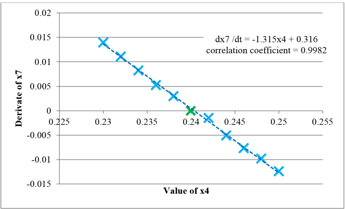
Figure 1: Example linear regression calculating element {\bf A}_{7,4} with a value of -1.315, with a correlation coefficient of 0.9982. The equilibrium point is shown in green
图 1：示例线性回归计算单元 ${\bf A}_{7,4}$，其值为 -1.315，相关系数为 0.9982。平衡点以绿色显示。 Last updated 30-08-2024

Multi-blade Coordinate Transformation

For linearisation calculations or Campbell diagrams it is recommended to select the multi-blade coordinate transformation, which generates coupled modes referring to the non-rotating coordinate system including the backward and forward whirling modes of the rotor. This is based on theory developed in (Bir, 2008) and (Hansen, 2003). The linearised model is significantly azimuth-dependent, but when transformed to non-rotating coordinates the resulting model of the structural dynamics should be only weakly azimuth-dependent. However, for 2-bladed turbines there is still a strong azimuth dependency.
为了线性化计算或坎贝尔图的绘制，建议选择多叶片坐标变换，该变换会生成与非旋转坐标系耦合的模态，包括风轮的后向和前向挥舞模态。这基于 (Bir, 2008) 和 (Hansen, 2003) 中提出的理论。线性化后的模型对方位角高度依赖，但当变换到非旋转坐标系后，结构动力学模型应仅表现出微弱的方位角依赖性。然而，对于2叶片风轮，仍然存在较强的方位角依赖性。

Single mode transformation

The transformation matrix of displacements of a 3-blade system with azimuths \psi_{1} to \psi_{3} from nonrotating to rotating coordinates is given by
一个三叶片系统，其方位角为 \psi_{1} 到 $\psi_{3}$，从非旋转坐标系到旋转坐标系的位移变换矩阵如下：

\begin{align}
\begin{bmatrix}
q_{1} \\
q_{2} \\
q_{3} \\
\end{bmatrix} &= \widetilde{{t}}_{NR \rightarrow R}
\begin{bmatrix}
q_{0} \\
q_{c} \\
q_{s} \\
\end{bmatrix},
\end{align}

with

\tilde{\mathbf{t}}_{N R\to R}=\left[\begin{array}{l l l}{1}&{\cos\psi_{1}}&{\sin\psi_{1}}\\ {1}&{\cos\psi_{2}}&{\sin\psi_{2}}\\ {1}&{\cos\psi_{3}}&{\sin\psi_{3}}\end{array}\right].

Multi-blade coordinate transformations are often quoted in the above form, but the primary aim is to go the other way and transform from rotating to non-rotating coordinates. The transformation matrix of displacements of a 3-blade system from rotating to non-rotating coordinates is the inverse of the above matrix given by
多叶片坐标变换通常以上述形式引用，但主要目的是反向变换，从旋转坐标系变换到非旋转坐标系。一个3叶片系统的位移从旋转坐标系变换到非旋转坐标系的变换矩阵，是上述矩阵的逆矩阵，由以下给出：

\begin{align}
{t}_{R \rightarrow NR} = \frac{1}{3}\begin{bmatrix}
1 & 1 & 1 \\
2\cos\psi_{1} & 2\cos\psi_{2} & 2\cos\psi_{3} \\
2\sin\psi_{1} & 2\sin\psi_{2} & 2\sin\psi_{3} \\
\end{bmatrix}.
\end{align}

Note, that the inverse relation does not hold for the derivatives of this matrix.

The general transformation matrix for a turbine with an arbitrary number of blades (n)
注意，此矩阵的导数不满足逆关系。

对于具有任意数量叶片 (n) 的风轮的通用变换矩阵

\mathbf{t}_{R\rightarrow N R}=\frac{1}{n}\left[\begin{array}{c c c c c}{1}&{1}&{1}&{\cdots}&{1}\\ {2\cos\psi_{1}}&{2\cos\psi_{2}}&{2\cos\psi_{3}}&{\cdots}&{2\cos\psi_{n}}\\ {2\sin\psi_{1}}&{2\sin\psi_{2}}&{2\sin\psi_{3}}&{\cdots}&{2\sin\psi_{n}}\\ {2\cos j\psi_{1}}&{2\cos j\psi_{2}}&{2\cos j\psi_{3}}&{\cdots}&{2\cos j\psi_{n}}\\ {2\sin j\psi_{1}}&{2\sin j\psi_{2}}&{2\sin j\psi_{3}}&{\cdots}&{2\sin j\psi_{n}}\\ {\vdots}&{\vdots}&{\vdots}&{\ddots}&{\vdots}\\ {1}&{-1}&{1}&{\cdots}&{(-1)^{n}}\end{array}\right],

where the last row is the transformation to the differential mode and exists only if there is an even number of blades. For odd bladed turbines, the last row will be a sine cyclic row. The counter j goes from 1 to (n-1)/2 if n is odd, and from 2 to (n-2)/2 if {n} is even.

Dropping the matrix representation the non-rotating coordinates can be calculated as

其中最后一行是变换到微分模态，且仅在叶片数量为偶数时存在。对于叶片数量为奇数的风轮，最后一行将是一个正弦循环行。计数器 j 从 1 到 (n-1)/2 (当 n 为奇数时)，从 2 到 (n-2)/2 (当 {n} 为偶数时)。

省略矩阵表示，非旋转坐标可以计算如下：

\begin{array}{l}{\displaystyle q_{0}=\frac{1}{n}\sum_{i=1}^{n}q_{i}}\\ {\displaystyle q_{c j}=\frac{2}{n}\sum_{i=1}^{n}q_{i}\cos{\left(j\psi_{i}\right)}}\\ {\displaystyle q_{s j}=\frac{2}{n}\sum_{i=1}^{n}q_{i}\sin{\left(j\psi_{i}\right)}}\\ {\displaystyle q_{d}=\frac{1}{n}\sum_{i=1}^{n}q_{i}(-1)^{n}}\end{array}

Returning to the specific case of 3-bladed turbines as an example, the derivative transformation matrices are now calculated. Each azimuth angle \psi_{i} can be expressed in terms of the (assumed constant) rotor speed \Omega and initial azimuth angle \Psi_{i} as linear relationship

以三叶风轮为例，现在计算导数变换矩阵。每个方位角 \psi_{i} 可以表示为（假设恒定的）风轮转速 \Omega 和初始方位角 \Psi_{i} 的线性关系。

\psi_{i}=\Omega t+\Psi_{i}.

Taking the time-derivatives of the transformation matrix gives 对变换矩阵求时间导数，得到：

\begin{align*}
\dot{{t}}_{R \rightarrow NR} =
\frac{\Omega}{3}
\begin{bmatrix}
0 & 0 & 0 \\
- 2\sin\psi_{1} & - 2\sin\psi_{2} & - 2\sin\psi_{3} \\
2\cos\psi_{1} & 2\cos\psi_{2} & 2\cos\psi_{3} \\
\end{bmatrix}
\end{align*}

and

\begin{align*}
\ddot{{t}}_{R \rightarrow NR} =
- \frac{\Omega^{2}}{3}
\begin{bmatrix}
0 & 0 & 0 \\
2\cos\psi_{1} & 2\cos\psi_{2} & 2\cos\psi_{3} \\
2\sin\psi_{1} & 2\sin\psi_{2} & 2\sin\psi_{3} \\
\end{bmatrix}
\end{align*}

for the first and second derivatives, respectively.

System transformation matrix

A transformation matrix for the whole state list, including both displacement and velocity states, is required. For the displacement states we have already established in Equation (1) that

需要一个包含位移和速度状态的整个状态列表的变换矩阵。正如我们在公式(1)中已经确立的，对于位移状态，

{\bf q}_{N R}={\bf t}_{R\rightarrow N R}{\bf q}_{R}

holds. Taking the time-derivative of Equation (1) gives 对公式(1)求时间导数，得到：

\dot{\bf q}_{N R}={\bf t}_{R\rightarrow N R}\dot{\bf q}_{R}+\dot{\bf t}_{R\rightarrow N R}{\bf q}_{R}

for the velocity states.

Combining {\bf q}_{N R} and \dot{\bf q}_{N R} to a vector of all states (both displacements and velocities) allows us to define a common transformation matrix \mathbf{T} that is of the same dimensions as A. We define

将 {\bf q}_{N R} 和 \dot{\bf q}_{N R} 组合成一个包含所有状态（位移和速度）的向量，允许我们定义一个与 A 具有相同维度的公共变换矩阵 $\mathbf{T}$。 我们定义

\begin{align}

{T} &:= \begin{bmatrix}

{t}_{R \rightarrow NR} & 0 \\

\dot{{t}}_{R \rightarrow NR} & {t}_{R \rightarrow NR} \\

\end{bmatrix}

\end{align}

allowing us to express the combined vector as

\begin{align}
\begin{bmatrix}
    q_{NR} \\
    \dot{q}_{NR}
\end{bmatrix}
&=
\begin{bmatrix}
    t_{R \rightarrow NR} & 0 \\
    \dot{t}_{R \rightarrow NR} & t_{R \rightarrow NR}
\end{bmatrix}
\begin{bmatrix}
    q_{R} \\
    \dot{q}_{R}
\end{bmatrix}.
\end{align}

Note that in general the displacement and velocity states are not ordered in this way and a permutation of the system transformation matrix \mathbf{T} will occur. The system transformation matrix is not singular and the inverse can be calculated.

The derivative of the system transformation matrix is trivially inferred as

需要注意的是，一般来说，位移和速度状态并非以这种方式排列，系统变换矩阵 \mathbf{T} 会发生置换。系统变换矩阵非奇异，可以计算其逆矩阵。

系统变换矩阵的导数可以很容易地推导出来。

\begin{align}

\dot{{T}}=

\begin{bmatrix}

\dot{{t}}_{R \rightarrow NR} & 0 \\

\ddot{{t}}_{R \rightarrow NR} & \dot{{t}}_{R \rightarrow NR} \\

\end{bmatrix}.

\end{align}

Transforming the A,B,C,D matrices

We consider the linear model equations in the rotating frame of reference and define
我们考虑在旋转参考系中的线性模型方程，并定义：

\begin{align}

{x}_{R} := \begin{bmatrix}

{q}_{R} \\ \dot{{q}}_{R}

\end{bmatrix}

\end{align}

to express the principal system as 为了表达主要系统为

\begin{array}{r}{\dot{\mathbf{x}}_{R}=\mathbf{A}_{R}\mathbf{x}_{R}+\mathbf{B}_{R}\mathbf{u}}\\ {\mathbf{y}=\mathbf{C}_{R}\mathbf{x}_{R}+\mathbf{D}_{R}\mathbf{u}}\end{array}

with respect to rotating blade coordinates.

The transformation of the state vector from rotating to non-rotating coordinates is given as
相对于旋转叶片坐标系。

状态向量从旋转坐标系变换到非旋转坐标系的表达式如下：

\mathbf{x}_{N R}=\mathbf{T}\mathbf{x}_{R}

and its derivative follows as

\dot{{\bf x}}_{N R}={\bf T}\dot{\bf x}_{R}+\dot{\bf T}{\bf x}_{R}.

By combining Equation (17) with Equation (15) we infer

\begin{array}{r l}&{\dot{\mathbf{x}}_{N R}=\mathbf{T}\left(\mathbf{A}_{R}\mathbf{x}_{R}+\mathbf{B}_{R}\mathbf{u}\right)+\dot{\mathbf{T}}\mathbf{x}_{R}}\\ &{\qquad=\Big(\mathbf{T}\mathbf{A}_{R}+\dot{\mathbf{T}}\Big)\mathbf{x}_{R}+\mathbf{T}\mathbf{B}_{R}\mathbf{u}}\\ &{\qquad=\Big(\mathbf{T}\mathbf{A}_{R}+\dot{\mathbf{T}}\Big)\mathbf{T}^{-1}\mathbf{x}_{N R}+\mathbf{T}\mathbf{B}_{R}\mathbf{u}}\end{array}

and conclude

\begin{array}{r l}&{\mathbf{A}_{N R}=\Big(\mathbf{TA}_{R}+\dot{\mathbf{T}}\Big)\mathbf{T}^{-1}}\\ &{\mathbf{B}_{N R}=\mathbf{TB}_{R}}\end{array}

from there.

Similar transformation in Equation (16) gives

\begin{array}{r}{\mathbf{y}=\mathbf{C}_{R}\mathbf{x}_{R}+\mathbf{D}_{R}\mathbf{u}}\\ \\{=\mathbf{C}_{R}\mathbf{T}^{-1}\mathbf{x}_{N R}+\mathbf{D}_{R}\mathbf{u}}\end{array}

for the output y of the linear system. We now define

\mathbf{C}_{N R}:=\mathbf{C}_{R}\mathbf{T}^{-1},\quad\mathrm{~and~}\mathbf{D}_{N R}:=\mathbf{D}_{R}

for the matrices concerned with the output of the linear model. This completes the derivation of a linear model with respect to a non-rotating frame

Rotational transformations are exclusively applied to states, which represent the degress of freedom in a mathematical model defined for all blades. These states include blade mode states as well as dynamic stall states, whereas any other individual-blade states such as pitch positions, rates, actuator internal states etc. are not transformed. The matrix T just has unit diagonal elements for rows and columns corresponding to the states and state derivatives which are not transformed. For other rows and columns, the elements of T represent the basic transformation defined above for each group of modes. Note that the elements connecting states and state derivatives also need to be defined by differentiating the equations of the basic transformation, bearing in mind that the derivative of the azimuth angle is equal to the rotor speed (which is assumed constant for this purpose). Model inputs and outputs are not transformed.
对于与线性模型输出相关的矩阵，本部分内容完成了对非旋转参考系下的线性模型推导。

旋转变换仅应用于状态，这些状态代表了定义在所有叶片上的数学模型中的自由度。这些状态包括叶片模态和动态失速状态，而其他任何单个叶片状态，例如桨距角位置、速率、执行器内部状态等，均不进行变换。矩阵 T 在未进行变换的状态和状态导数对应的行和列上具有单位对角线元素。对于其他行和列，T 的元素代表上述为每组模态定义的基变换。需要注意的是，连接状态和状态导数的元素也需要通过对基变换方程进行微分来定义，同时考虑到方位角的变化率等于风轮转速（出于本目的，假设其为常数）。模型输入和输出不进行变换。

Last updated 26-11-2024

Coupled Modes

Calculating Coupled Modes

The Campbell diagram and blade stability analyses are analyses of the matrix A at each specified operating point. Each coupled mode corresponds to an eigenvalue and its eigenvector. Given a (complex) eigenvalue, \lambda, of A, Bladed reports the undamped frequency \displaystyle(\omega_{n}), damped frequency ( \omega_{d} ) and damping ratio (\zeta) according to Figure 1.

坎贝尔图和叶片稳定性分析是对在每个指定工作点处的矩阵 A 的分析。每个耦合模态对应一个特征值及其特征向量。给定矩阵 A 的一个（复数）特征值 λ，Bladed 会根据图 1 报告无阻尼频率undamped frequency (ωn)、阻尼频率damped frequency (ωd) 和阻尼比 (ζ)。

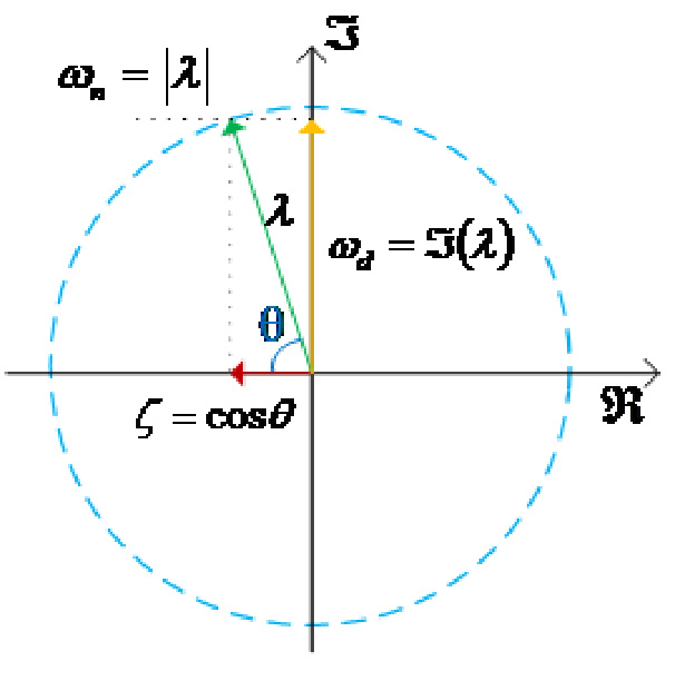
Figure 1: Argand Diagram阿根图

The uncoupled mode contributions to each coupled mode are determined by its eigenvector. If the coupled mode has contributions from second-order states (structural states), which are represented by two states in the state vector, then the displacement state is used to determine the contribution.

In their raw form, these eigenvector contributions represent the relative displacement of each mode and can be used to build up the coupled mode-shape. However, the contributions in the Campbell diagram have been normalised. This is done by modifying the matrix of eigenvectors such that each row and each column have a unit sum. This has the effect of increasing percentage contributions from modes with high mass and stiffness, which contribute very little in displacement but significantly in energy.

The phase of each contribution, \phi_{i\,,} is determined by the argument of the corresponding complex eigenvector element, v_{i}, i.e.

每个耦合模态的未耦合模态贡献由其本征向量决定。如果耦合模态具有二阶状态（结构状态）的贡献，这些状态由状态向量中的两个状态表示，则使用位移状态来确定贡献。

以原始形式，这些本征向量贡献代表每个模态的相对位移，可用于构建耦合模态形状。然而，在坎贝尔图中，这些贡献已被归一化。这是通过修改本征向量矩阵来实现的，使得每一行和每一列都具有单位和。这会增加具有高质量和刚度的模态的百分比贡献，这些模态在位移中贡献很小，但在能量方面贡献很大。

每个贡献的相位，\phi_{i\,,} 由相应复本征向量元素的参数决定，即 v_{i}, 即。

\phi_{i}=\arctan\left(\frac{\operatorname{Im}\left(v_{i}\right)}{\operatorname{Re}\left(v_{i}\right)}\right).

Last updated 26-11-2024

Naming Coupled Modes

In cases where coupled modes are computed such as in the Campbell diagram analysis the following sections gives details on the naming. A focus is placed on the behaviour when the multiblade coordinate transform is used.
在计算耦合模态，例如在坎贝尔图分析中，以下章节将详细介绍命名规范。重点关注多叶片坐标变换使用时的行为。

Support structure modes

For support structure modes, the coupled mode is named after the whole-tower mode that gives the highest contribution. Whole-tower modes are uniquely calculated for the linearisation calculations through a subsequent eigen analysis with fixed-free boundary conditions. This analysis considers the effect of the RNA and any other masses at distal nodes. In case multiple coupled support structure modes share the same whole-tower mode as its prime contributor, then the coupled mode name is made unique by appending letters A,B,C, and so on.
对于支撑结构模态，耦合模态以对贡献最大的整个塔架模态命名。整个塔架模态通过后续带有固定-自由边界条件的特征分析来计算，用于线性化计算。该分析考虑了RNA（叶片）以及位于远端节点上的其他质量的影响。如果多个耦合支撑结构模态共享相同的整塔模态作为其主要贡献者，则通过附加字母A、B、C等来使耦合模态名称唯一化。

Rotor modes rotating frame

If no MBC(Multi-blade Coordinate) transformation is used for the rotor modes, then the following logic applies to naming the coupled rotor modes:

· If a single blade mode gives >\!75\% contribution to the coupled rotor mode, then the coupled rotor mode is named after that blade mode. In other words, the mode is called "Blade" instead of "Rotor" mode.
· Else, the rotor mode is named after its prime contributor and made unique by appending letters \mathsf{A},\mathsf{B},\mathsf{C}, etc. in case multiple coupled rotor modes share the same uncoupled blade mode as prime contributor

如果未使用多叶片坐标变换(MBC)来描述风轮模态，则以下逻辑适用于命名耦合风轮模态：

· 如果单个叶片模态贡献超过75%，则将耦合风轮模态命名为该叶片模态。换句话说，该模态被称为“叶片”模态，而不是“风轮”模态。 · 否则，耦合风轮模态以其主要贡献者命名，并通过附加字母A、B、C等来使其独一无二，以防多个耦合风轮模态共享相同的未耦合叶片模态作为主要贡献者。

Rotor modes non-rotating frame

If an MBC transform is applied then the individual blade modes are transformed to a set of rotor modes. For a three bladed rotor there typically is a collective, cosine-cyclic and sine-cyclic rotor mode. The 1st flapwise modes of all blades will be renamed to rotor 1st flapwise collective, rotor 1st flapwise sine-cyclic and rotor 1st flapwise cosine cyclic. In case the number of blades is even there will be a differential mode as well.

After the transformation and renaming of the individual blade modes the coupled rotor modes are named. The whirling modes are identified following the logic in the table below.

Coupled mode name 1st uncoupled mode 2nd uncoupled mode Phase angle (\phi_{2}-\phi_{1})

如果应用了 MBC 变换，则各个叶片模态将被转换成一组风轮模态。对于三叶风轮，通常存在集变模态collective、余弦循环模态cosine-cyclic和正弦循环sine-cyclic模态。所有叶片的 1 阶挥舞模态将被重命名为风轮 1 阶挥舞集变模态、风轮 1 阶挥舞正弦循环模态和风轮 1 阶挥舞余弦循环模态。如果叶片数量为偶数，则还会存在摆振模态。

在转换和重命名各个叶片模态之后，命名耦合风轮模态。旋转模态的识别遵循下表中的逻辑。

Coupled mode name	1st uncoupled mode	2nd uncoupled mode	Phase angle (\phi_{2}-\phi_{1}))
Forward whirl	Sine cyclic	Cosine cyclic	> 0.0
	Cosine cyclic	Sine cyclic	< 0.0
Backward whirl	Sine cyclic	Cosine cyclic	< 0.0
	Cosine cyclic	Sine cyclic	> 0.0

If a coupled mode does not meet the criteria of the whirling modes, then the mode is named after its prime contributor. This is analogous with the naming logic of rotor modes in the rotating frame and support structure modes
如果一个耦合模态不符合颤动模态的标准，则该模态会被命名为其主要贡献者的名称。这与风轮在旋转参考系中的模态以及支撑结构模态的命名逻辑类似。

Last updated 04-12-2024

Joining Coupled Modes across Operating Points 连接不同工况下的耦合模态

The Campbell diagram displays the frequencies of different coupled displacement modes with respect to the rotor speed together with the most important excitation frequencies given in terms of multiples of the rotor frequency (P). In addition to the frequencies of the coupled modes, the Campbell diagram displays the corresponding damping ratios, which include the effect of structural damping as well as aerodynamic damping. Both characteristics are calculated as described in the article Calculating Coupled Modes and are useful for identifying the critical Operating points that need further analysis.

坎贝尔图显示了不同耦合位移模态相对于风轮转速的频率，以及以风轮频率（P）的倍数给出的最重要激励频率。 除了耦合模态的频率，坎贝尔图还显示了相应的阻尼比，其中包括结构阻尼和气动阻尼的影响。 这两个特征的计算方法如文章“Calculating Coupled Modes”中所述，可用于识别需要进一步分析的关键运行点。

The Joining Process连接过程

Given a set of coupled modes at each operating point, a fundamental step in creating the resulting Campbell diagram is to identify similar modes at adjacent operating points, which allows for joining similar modes across the operating points with line segments, giving the user the impression of continuous change in frequency against rotor speed (or wind speed). This joining process is generally challenging because the coupled modes evolve and change in their contributions between the operating points.

Similar coupled modes at two adjacent operating points are identified by comparing their complex eigenvectors and frequency in term of the extended modal assurance criterion (MACX) (Vacher, Jacquier, and Buchales, 2010) with frequency weighting. More specifically, the frequency weighted MACX numbers are calculated for all combinations of coupled modes at the two operating points to form a score matrix, which are then used for joining the modes by the GaleShapley algorithm (Gale & Shapley, 1962). A sequence of similar modes at all operating points forms a coupled mode series, which represents a line in the resulting Campbell diagram.

To ensure that the coupled mode series in the resulting Campbell diagram primarily involves structural dynamics, an initial calculation of coupled modes with only structural states is performed at the first operating point. These structure-only modes are then joined with the coupled modes at the first operating point as described above, which effectively excludes coupled modes that mainly have contributions from aerodynamic states.

给定一组在每个工作点耦合的模态，创建最终的坎贝尔图的关键步骤是识别相邻工作点中相似的模态，这使得能够用线段连接这些相似的模态，从而给用户留下频率随风轮转速（或风速）连续变化的印象。这种连接过程通常具有挑战性，因为耦合模态在工作点之间会演变和改变其贡献。

通过比较在扩展模态保证准则（MACX）（Vacher, Jacquier, 和 Buchales, 2010）下的复特征向量和频率，并采用频率加权，可以识别出两个相邻工作点中的相似耦合模态。更具体地说，会为两个工作点中所有耦合模态组合计算频率加权 MACX 数值，形成一个评分矩阵，然后使用该矩阵通过 GaleShapley 算法（Gale & Shapley, 1962）连接这些模态。所有工作点中一系列相似的模态构成一个耦合模态序列，它代表了最终坎贝尔图中的一条线。

为了确保最终坎贝尔图中的耦合模态序列主要涉及结构动力学，在第一个工作点执行一次仅包含结构状态的耦合模态计算。然后，将这些仅结构模态与如上所述的第一个工作点的耦合模态连接起来，这有效地排除了主要来自气动状态贡献的耦合模态。

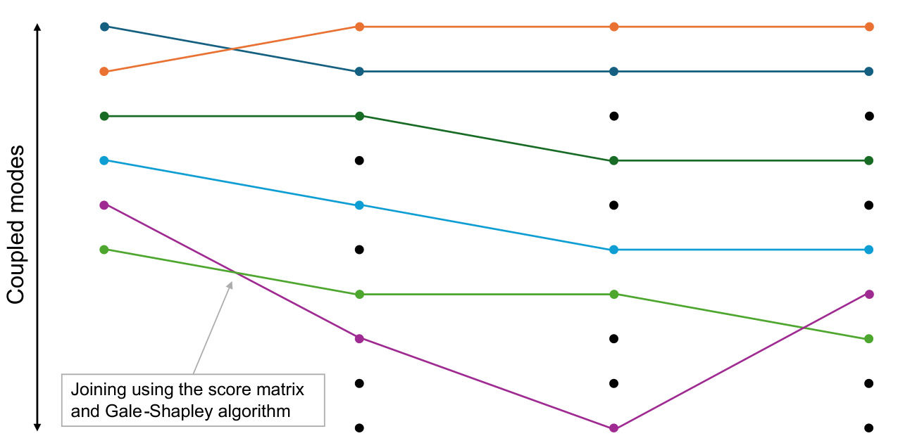
Figure 1: Illustration of the joining process showing how the coupled modes are connected at the operating points. Dots represent coupled modes. Coloured lines represent coupled mode series. 图 1：连接过程示意图，展示了耦合模态在工作点处的连接方式。点代表耦合模态。彩色线条代表耦合模态级数。

The resulting joining process is then:

1. Calculate a set of structure-only modes at the first operating point. These modes will also form the basis of the mode series, representing the lines in the resulting Campbell diagram.
2. Join the structure-only modes with the coupled modes at the first operating point. It is noted that the number of coupled modes is generally larger than the number of mode series, which means that not all coupled modes are included in a mode series.
3. Join the coupled modes that were included in a mode series at the current point (first operating point) with the coupled modes at the next point (second operating point). Repeat until the last operating point is reached.

接下来的连接过程如下：

4. 计算在第一个工作点的一组仅结构模态。这些模态也将构成模态序列的基础，代表最终的坎贝尔图中的线。
5. 将仅结构模态与在第一个工作点的耦合模态连接起来。需要注意的是，耦合模态的数量通常大于模态序列的数量，这意味着并非所有耦合模态都包含在模态序列中。
6. 将在当前点（第一个工作点）包含在模态序列中的耦合模态与下一个点（第二个工作点）的耦合模态连接起来。重复此过程直至到达最后一个工作点。

Naming and Exclusion of Coupled Mode Series

A coupled mode series is named according to the contributions of the structure-only coupled modes at the first operating point only (more details on coupled mode naming can be found here). The contributions and therefore the shape of a coupled mode can change significantly between the range of operating points, and therefore the characteristic of a mode cannot be determined from the name alone.

A coupled mode series, which includes coupled modes with real eigenvalues (and therefore no oscillatory behaviour) at all operating points, is excluded from the resulting Campbell diagram. This is done because such modes cannot cause resonant behaviour, which is the primary purpose of the Campbell diagram to detect.

A coupled mode series is also excluded if the coupled mode frequencies at all operating points exceed a user-defined maximum value.

一种耦合模态级数，仅根据第一个工作点处的结构-模态耦合贡献来命名（关于耦合模态命名的更多细节请参见此处）。耦合模态的贡献，因此其形状，在工作点范围的不同情况下可能会发生显著变化，因此仅凭名称无法确定模态的特性。

一种耦合模态级数，其中包含所有工作点处具有实特征值（因此没有振荡行为）的耦合模态，将被排除在最终的坎贝尔图之外。这是因为此类模态无法引起共振行为，而坎贝尔图的主要目的是检测共振行为。

如果所有工作点处的耦合模态频率超过用户定义的上限值，则该耦合模态级数也会被排除。

Last updated 26-11-2024

Align Wind Field with Hub Axis

Figure 1 illustrates that azimuthal dependency is still invoked in certain cases even though the considerations given in the linear analysis background are followed. This occurs when a tilt angle is considered in the calculations and when the tower flexibility is strongly affecting the rotor orientation. Figure 1 (left) provides an ilustration of the azimuthally independent system, indicating that the solution will be the same regardless of the azimuth angle of the rotor. However, when the tilt angle is considered, Figure 1 (middle), the loads perceived by the upper side of the rotor and the lower side of the rotor vary. This creates an imbalance of the loads similar as adding "a virtual wind shear" on the rotor plane. The situation is worse when the flexibility of the tower affects the rotor orientation strongly as illustrated in Figure 1 (right). Here, one can see that the hub orientation might be tilted even greater which creates a stronger loads imbalance across the rotor.

图1所示，即使遵循线性分析背景中的考虑因素，在某些情况下仍然需要调用方位角依赖性。当计算中考虑倾角，且塔架柔度强烈影响风轮姿态时，这种情况会发生。图1（左）提供了一个方位角独立的系统示意图，表明无论风轮的方位角角度如何，解都是相同的。然而，当考虑倾角时，如图1（中间）所示，风轮上部和下部受到的载荷会发生变化。这会产生类似于在风轮平面上添加“虚拟风切变”的载荷不平衡。当塔架柔度强烈影响风轮姿态时，情况会更加糟糕，如图1（右）所示。在这里，可以看到轮毂姿态可能会倾斜得更大，从而在风轮上产生更强的载荷不平衡。

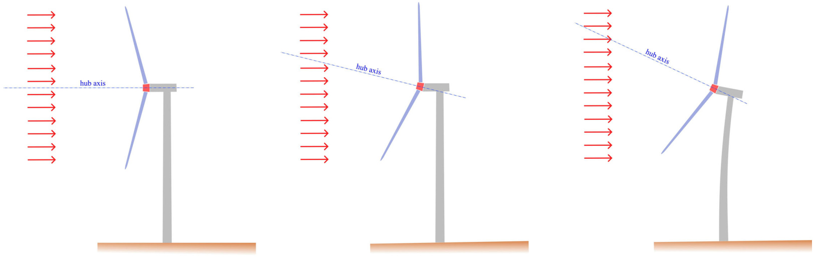
Figure 1: llustration of the hub axis orientation relative to the incoming wind direction in the linearisation calculation. Left: rigid wind turbine without tilt angle, middle: rigid wind turbine with tilt angle being considered, right: flexible turbine with tilt angle being considered.
图1：线性化计算中，风轮轴向相对于迎风方向的示意图。左：无倾角刚性风轮，中：考虑倾角的刚性风轮，右：考虑倾角的柔性风轮。

To avoid the imbalance of the loads due to the tilted hub orientation, Bladed introduces a correction to align the wind field according to the tilted hub axis orientation. The mechanism is clearly illustrated in Figure 2. It can be observed that when the wind field is aligned with the tilted hub axis, the loads experienced by the rotor will be independent of the azimuth angle. This effectively removes the azimuthal dependency of the system due to tilted hub axis orientation. This correction may also be applied for floating wind turbines as illustrated in Figure 3.

为了避免倾斜轴向导致的载荷不平衡，Bladed 引入了一种校正措施，以使风场与倾斜轴向对齐。该机制在图2中清晰地说明。可以观察到，当风场与倾斜轴向对齐时，风轮受到的载荷将与偏航角无关。这有效地消除了由于倾斜轴向引起的系统偏航角依赖性。 这种校正也可以应用于浮式风力发电机，如图3所示。

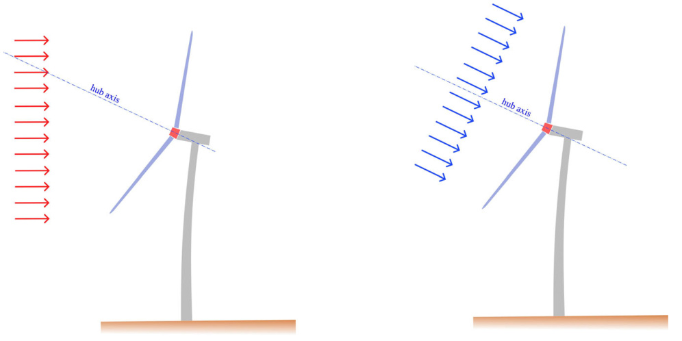
Figure 2: Aligning wind field to the tilted hub axis orientation for an onshore wind turbine or a bottom-fixed offshore wind turbine. Left: Azimuthally dependent system, right: azimuthally independent system.
图2：针对陆上风力发电机或固定基础海上风力发电机，将风场对准倾斜的轴向。左：方位角相关的系统，右：方位角无关的系统。

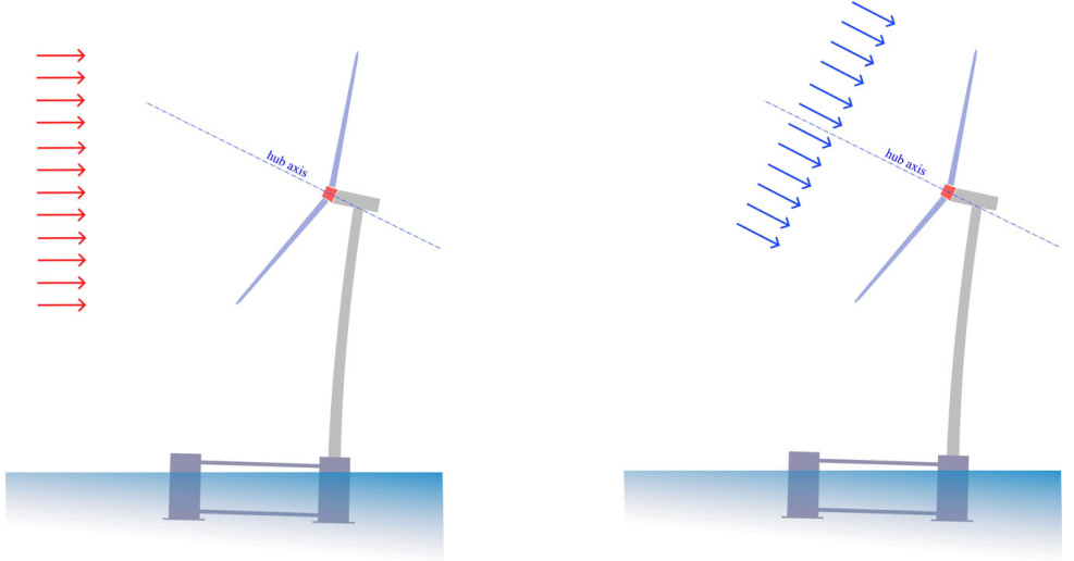
Figure 3: Aligning wind field to the tilted hub axis orientation for a floating wind turbine. Left: Azimuthally dependent system, right: azimuthally independent system.
图3：针对浮动式风力发电机，将风场对准倾斜的轴向。左：方位角相关的系统，右：方位角无关的系统。

The hub axis is determined during the initial conditions routine, where the rotor is not accelerating and the modal deflections are such that the elastic loads balance the external loading. Within the initial conditions routine, iterations are performed and the wind field is adjusted accordingly for every iteration to be parallel to the tilted hub axis. After the the conditions are found, the wind field orientation is fixed to the last found tilted angle in the initial conditions routine. Then, the system is perturbed using the fixed wind field orientation for calculating any of the linearisation type calculations available in Bladed. This process is done for every operating point simulated.

初始条件程序中确定风轮中心轴，此时风轮未加速，模态变形使得弹性载荷与外部载荷平衡。在初始条件程序中，进行迭代计算，并在每次迭代中调整风场，使其与倾斜的风轮中心轴平行。一旦找到合适的条件，风场方向就被固定在初始条件程序中最后确定的倾斜角度。随后，系统使用固定的风场方向进行扰动，用于计算Bladed中可用的任何线性化类型计算。此过程针对每个模拟的工作点进行。

Last updated 30-08-2024