60 KiB
About the Blades
This section provides descriptions of the various modelling options and definitions for simulating wind turbine blades. Bladed provides a versatile method of defining complex blade properties:
· The user can define a series of 2D blade sections along the neutral axes of the blade. At each section, a set of blade section coordinate systems are defined for structural and aerodynamic properties. This approach enables the possibility of defining aerofoil orientations and changing structural properties along the blade.
· An aerofoil library is provided, allowing for the definition of aerofoils that can be applied and interpolated at individual blade sections.
·Advanced flexibility options are available to accurately capture the non-linear nature of long and anisotropic blades. Options include a finite element model capable of modal reduction, a multi-part blade method for increased accuracy of large deflections and a geometric stiffness model to capture second-order effects.
· A suite of blade load outputs and kinematic outputs are provided in various blade coordinate systems.
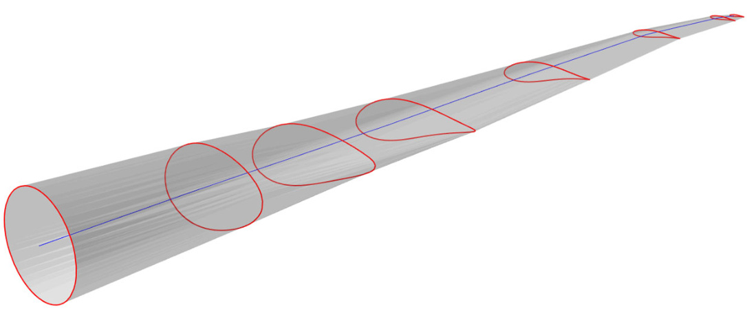
Figure 1: llustration of a typical wind turbine blade.
Last updated 13-12-2024
Blade Root and Neutral Axes Systems
In Bladed, the blade sections are defined as a finite series of 2D sections along the blade's span, using the neutral axes system relative to the blade root axes system.
Origin of Blade Root Axes System
The root axes coordinate system is a body-fixed coordinate system, which coincides with the blade root centre.

Figure 1: Blade root coordinate system, illustrated for zero cone and pitch.
The orientation of the blade root is influenced by properties inboard and outboard of the pitch bearing, as illustrated in Figure 2 and summarised in the table below. These properties determine the blade's mounting angles relative to the pitch axis. If no mounting sweep or cone angles are applied, the Blade root Z-axis aligns with the pitch axis. Non-zero angles for either Blade mounting cone angle or Blade mounting sweep angle create an orientation difference between the pitch and blade root Z-axis, as seen in Figure 2. All subsequent blade properties are defined relative to the Blade root Z-axis .
Table 1: Blade mounting properties and their effects on the blade root z-axis
<html>| Property | Location | Unit | Description |
| Cone angle | Inboard of pitch bearing | deg A positive angle cones the tip away from the nacelle. Defined in Rotor screen. | |
| Blade mounting cone angle | Outboard of pitch bearing | deg A positive angle cones the tip away from the nacelle. Defined in Blades screen. | |
| Blade mounting sweep angle | Outboard of pitch bearing | deg | Indicates how much the blade tip is swept back from the pitch axis, away from the rotation direction. Defined in Blades screen. |
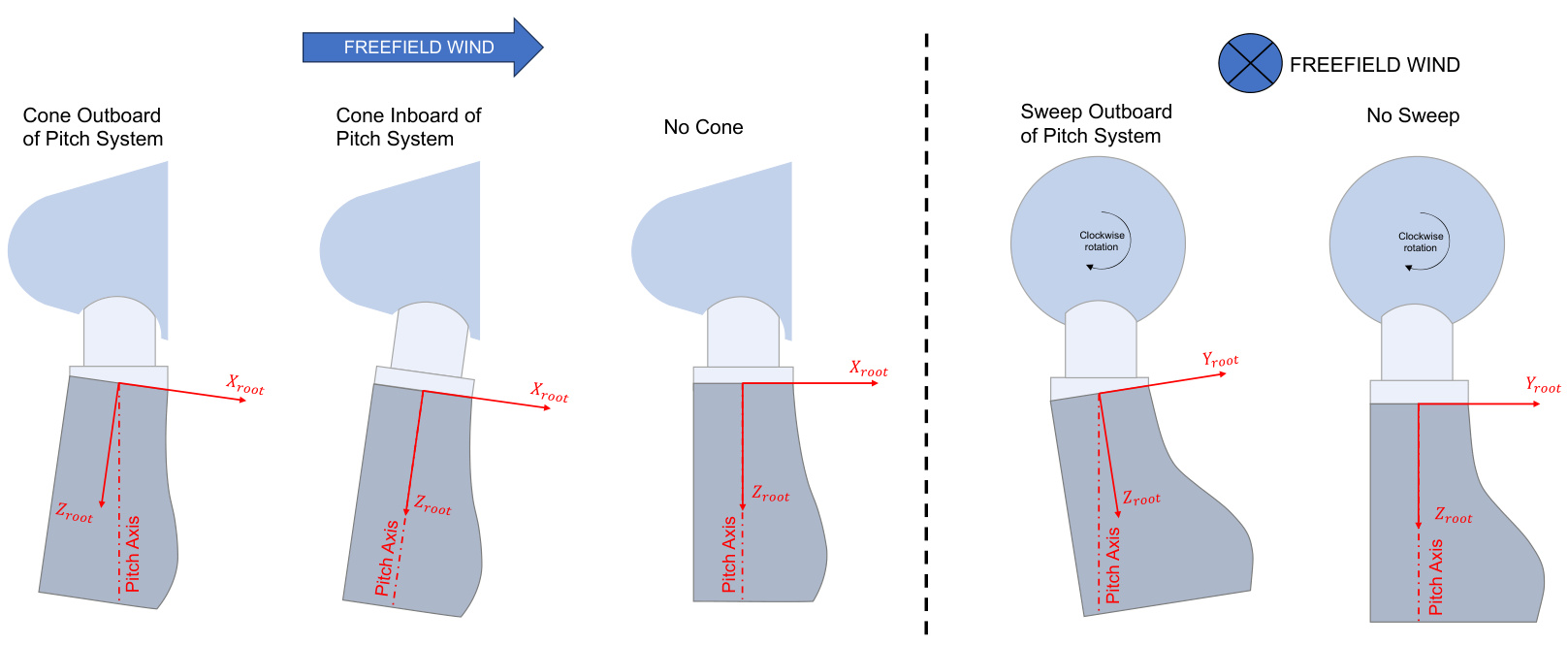
Figure 2: Left: Positive cone angle (inboard and outboard). Right: Positive sweep angle (outboard only, inboard not supported).
Blade Neutral Axes System
The neutral axis passes through the elastic centre of each blade section. Required inputs can be found in the Blades screen under the Blade Geometry and Mass and Stiffness tabs.
\textcircled{i} NOTE
The neutral axis is also commonly known as the principal elastic axis, bending axis, or simply the elastic axis.
The origin of the neutral axes system is defined using the following variables:
Neutral axis (x) Neutral axis (y)
All structural properties for the section, such as stiffness and mass, are then defined in specific blade section coordinate systems. The blade root and neutral axes system for a blade is showed in the figures below:
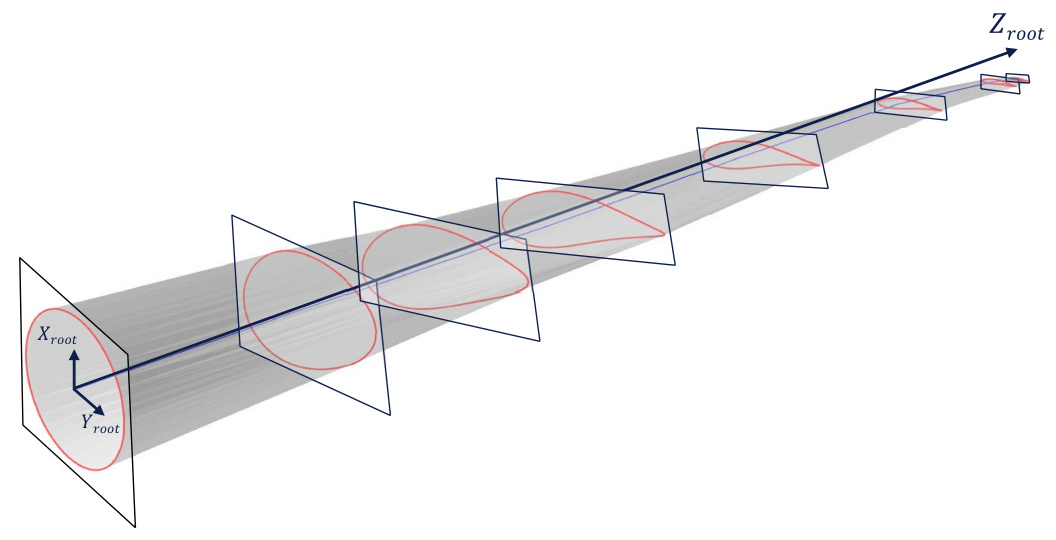
Figure 3: Blade root axes system and section planes
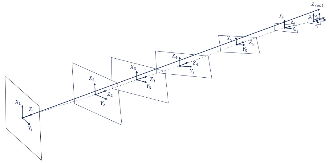
Figure 4: Blade neutral axes system and section planes
Distance Along Blade
Only one ofthe variables, Distance along blade or Distance along blade root Z-axis ,is needed to define the position of the neutral z-axis; the other is calculated automatically.
· Distance along blade root Z-axis refers to the position of the blade station along the blade rootZ-axis.
· Distance along blade is the cumulative distance from the blade root to the current blade station, along the blade neutral axis, which does not have to be a straight line. It must be zero for the first station.
\mathrm{DistanceAlongBlade}_{\mathrm{n}}=\sum_{i=1}^{n-1}\Delta d_{i+1,i}=\Delta d_{2,1}+\cdot\cdot+\Delta d_{n,n-1}
Where \Delta d_{i,j} is the distance between two section origins:
\Delta{d}_{i,j}=\left|\begin{array}{c}{{X_{0_{i}}-X_{0_{j}}}}\\ {{Y_{0_{i}}-Y_{0_{j}}}}\\ {{Z_{0_{i}}-Z_{0_{j}}}}\end{array}\right|
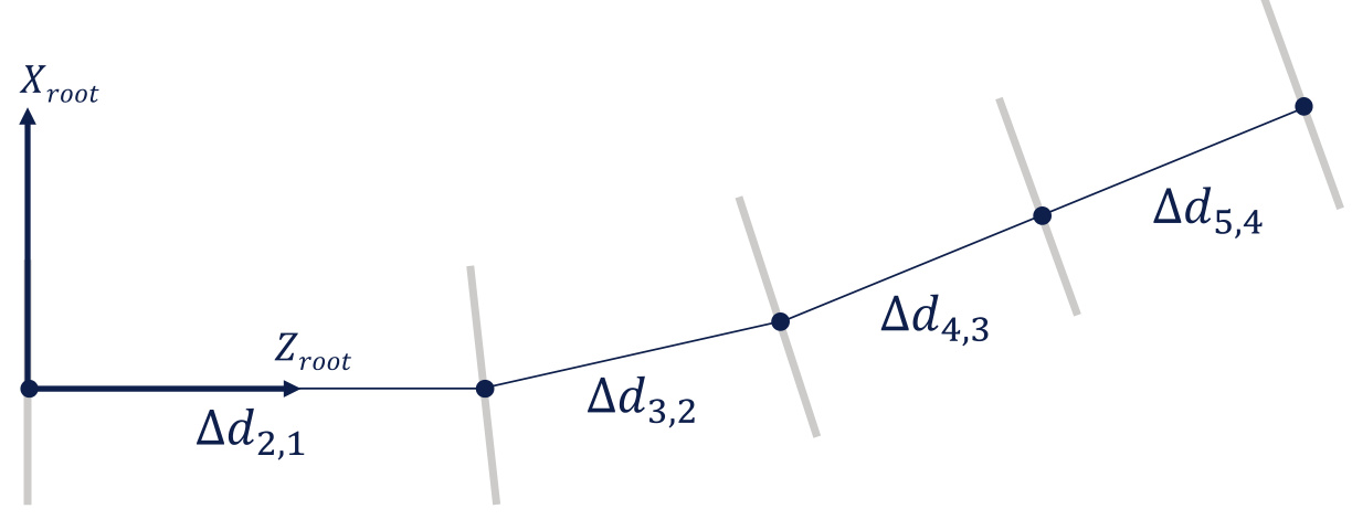
Figure 5: llustration of the Distance along blade definition
Last updated 13-12-2024
Blade Section Property Coordinate Systems
The blades in Bladed are defined as a finite series of 2D sections along the blade's span, using the neutral axes system relative to the blade root axes system.
Each section has an aerofoil that is oriented according to the Aerodynamic twist , with an associated chord axes system origin located at the leading edge as shown in Figure 1. The aerofoil must be positioned relative to the neutral z-axis, which passes through the elastic centre of each blade section. This is done by defining the location of the elastic centre as a percentage of the Chord length, measured from the aerofoil leading edge along the chord axes that follow the Aerodynamic twist :
Elastic centre (x') Elastic centre (y')
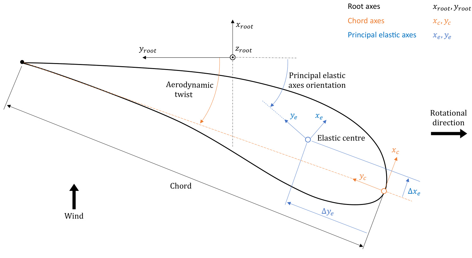
Figure 1: Blade section principal elastic axes coordinate system
Details on the orientation of the local element frame relative to the blade root axes can be found in Blade Local Element Axes.
Each section then allows for the definition of additional property systems that describe the structural and aerodynamic properties of the blade.
\textcircled{i} NOTE
Not all coordinate systems are relevant in every model; their inclusion depends on the model's complexity. For example, the principal shear axes coordinate system is not needed if Shear stiffness is omitted.
Coordinate
<html>| System | Description |
| Root axes | Fixed to the blade root, and it does not rotate with twist or blade deflection but rotates about the z-axis with pitch. |
| Chord axes | Located at the leading edge of the aerofoil and follows the Aerodynamic twist. |
| Principal elastic axes | Located at the Elastic centre and follows the Principal elastic axes orientation (xe, ye). |
| Principal shear axes | Located at the Shear centre and follows the Principal shear axes orientation (xs, ys) . |
| Principal inertia axes | Located at the Mass centre and follows the Principal inertia axes orientation (xm, ym) . |
| User axis | Located at the User axis , specified by the user for additional loads output. See Loads Outputs at User Axes for details. |
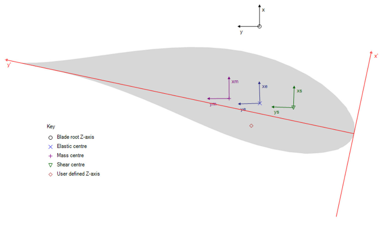
Figure 2: Overview of blade section coordinate systems in Bladed.
Definition of Centre Locations and Axes Orientations
The centres, including the Elastic centre, Shear centre, Mass centre and User axis,are all defined with respect to the chord axes, which are controlled by the Aerodynamic twist . The
locations of these centres are specified as a percentage of the chord length measured from the aerofoil leading edge. An example of this is illustrated in Figure 3 for the Shear centre definition.
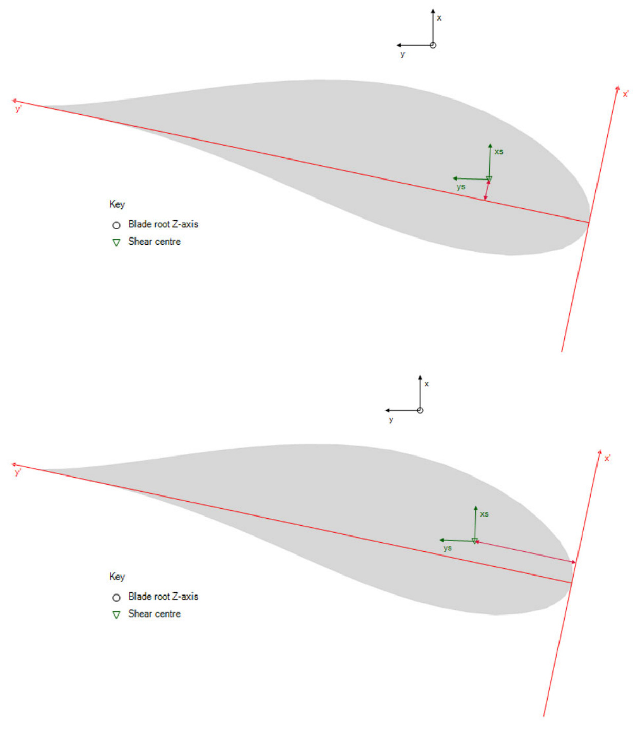
Figure 3: Top: Definition of shear centre (x'). Bottom: Definition of Shear centre (y').
Furthermore,the orientations of the Aerodynamic twist , Principal elastic axes orientation (xe, ye), Principal shear axes orientation (xs, ys),and Principal inertia axes orientation (xm, ym) are all defined with respect to the root axes and are positive in the clockwise direction as shown in Figure 4. In the GUl, the unit of the inputs is in degrees, whereas in the project file, it is in radians.
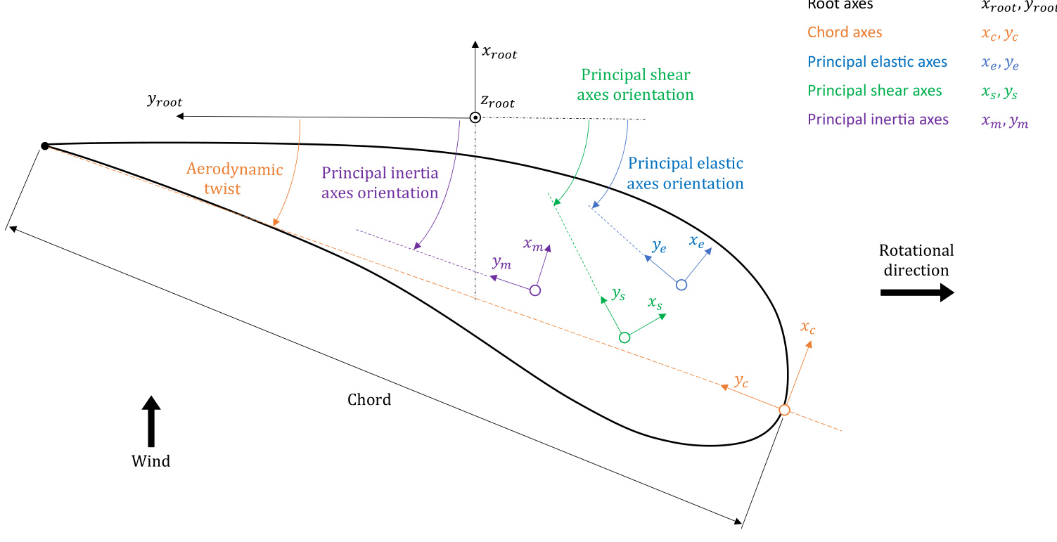
Figure 4: Definition of various property axes orientations in Bladed.
Overview of Blade Section Inputs and Associated Coordinate Systems
This section provides an overview of the structural properties defined in the various coordinate systems. For more details, see Blade Section Stiffness and Blade Section Mass.
Principal Elastic Axes
The following blade section input properties are defined in the principal elastic axes coordinate system:
Bending stiffness about xe
Bending stiffness about ye
Shear stiffness along xe
Shear stiffness along ye
Axial stiffness
FlapEdgeCStiff
TorsionFlapCStiff
TorsionEdgeCStiff
Principal Shear Axes
The following blade section input property is defined in the principal shear axes coordinate system:
Torsional stiffness
The following blade section input properties are defined in the principal inertia axes coordinate system:
Mass/unit length
Polar mass moment of inertia/unit length
Radii of gyration ratio
Chord Axes
The following blade section input properties are defined in the chord axes coordinate system:
Chord Thickness Foil section
Last updated 16-12-2024
Blade Section Geometry
The blade geometry is defined for each blade station. Select the option at the bottom of the screen to specify either the distance along blade or distance along blade root Z-axis .The alternate value will be automatically calculated using the neutral axis values. For example, selecting Distance along blade will automatically calculate the Distance along blade root Zaxis , and vice versa. For details refer to the section on Distance Along Blade. The following geometry data is required at each blade station:
Table 1: Overview over required geometry parameters for blade definition in Bladed
Variable identifier Unit Description
<html>| Distance along blade | m | The distance from the blade root to the current station along the neutral axis, which may not be straight. It must be zero for the first station. |
| Distance along blade root Z-axis | m | The distance of the blade station along the blade root Z-axis. |
| Chord | m | The distance from the leading edge to the trailing edge along the chord line. |
| Aerodynamic twist deg The local angle of the chord line. More positive values of twist and set angle push the leading edge further upwind in the direction from which the flow is coming. | ||
| Thickness | % | The thickness of the blade as a percentage of the chord at that station. |
| Neutral axis (x) | m | The distance from the blade root Z-axis to the neutral axis in the x- direction. This would be non-zero if, for example, the blade was pre- bent. |
| Neutral axis (y) | m | The distance from the blade root Z-axis to the neutral axis in the y- direction. |
| Elastic centre (x') | % | The distance from the leading edge to the elastic centre along the chord x-axis, as a percentage of the chord. |
| Elastic centre (y') | % | The distance from the leading edge to the elastic centre along the chord y-axis, as a percentage of the chord. |
| Foil section | An index number defining the aerofoil section at that station. | |
| Moving/Fixed | Differentiates between fixed and movable parts of the blade for pitch of that part of the blade, or by deploying an aileron, flap or other aerodynamic control surfaces. |
Figure 1 and Figure 2 illustrate a blade station for Clockwise and Anticlockwise rotor configurations. It is assumed that the perspective is from the tip toward the root, aligned to the root axes plane.
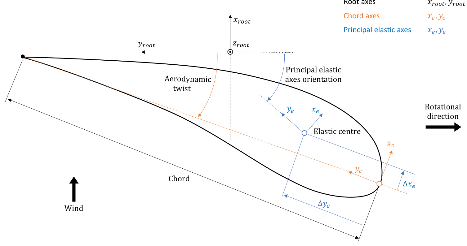
Figure 1: Aerofoil at a blade station illustrating root axes, principal elastic axes and chord axes.
Anticlockwise Rotors
The blade inputs for an Anticlockwise rotor use a left-handed coordinate system, in contrast to the right-handed system for clockwise rotors. As a result, no changes are needed to the input data when switching between Clockwise and Anticlockwise rotors. See Figure 2 for an illustration of the Anticlockwise blade definition.
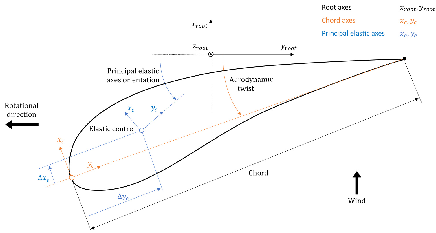
Figure 2: Anticlockwise rotating blade station, where the left-handed coordinate system ensures compatibility when switching between rotor directions.
Blade Section Stiffness
To model flexible blades or analyse vibrational dynamics, it is necessary to define the stiffness distribution of the rotor blade. Begin by selecting the appropriate degrees of freedom to include in the model by enabling/disabling the following options in the Blades screen under the Mass and Stiffnesstab:
Bending stiffness
Shear stiffness
Torsional degree of freedom
Axial degree of freedom
It is also possible to include bend-twist and bending-bending couplingterms, and these can be defined using Project info .
Constitutive Relationship
The blade sectional stiffness inputs all relate to the cross-sectional 6\!\times\!6 stiffness matrix used in the Bladed beam model as shown in Equation (1). This matrix is associated with the principal elastic axes coordinate system, which is defined by the Principal elastic axes orientation (xe, ye) and the Elastic centre as described in Blade Section Coordinate Systems. The constitutive relationship for the full beam model can be expressed as:
\left[\begin{array}{c}{F_{x}}\\ {F_{y}}\\ {F_{z}}\\ {M_{x}}\\ {M_{y}}\\ {M_{z}}\end{array}\right]=\left[\begin{array}{c c c c c c c}{G A_{x}}&&&&{\left|}&&&\\ {G A_{x y}}&&{G A_{y}}&&&{\left|}&&{\mathrm{sym}}\\ {0}&{0}&&{E A}&{\left|}&&&\\ {-}&{-}&{-}&{-}&{-}&{-}&{-}&{-}\\ {0}&{0}&{0}&{\left|}&{E I_{x}}&&\\ {0}&{0}&{0}&{\left|}&{C_{x y}}&{E I_{y}}\\ {-G A_{x}y_{c s}}&{G A_{y}x_{c s}}&{0}&{\left|}&{C_{x z}}&{C_{y z}}&{G I_{z}}\right.\right]\left[\kappa_{z}\right]
where
G I_{z}=G I_{z}^{*}+G A_{x}\cdot y_{c s}^{2}+G A_{y}\cdot x_{c s}^{2}
\mathbf{\boldsymbol{x}}_{c s} and y_{c s} are the offsets between the Elastic centre and shear centre along the principal elastic axes.
Table 1: Overview of blade sectional stiffness inputs in Bladed, relating them to Equation (1).
<html>| Property | Variable | Description | Unit | Input Location |
| Bending stiffness about xe | EIc | Bending stiffness about the principal elastic x-axis | Nm2 | Blades |
| screen | ||||
| Bending stiffness about ye | EIy | Bending stiffness about the principal elastic y-axis | Nm2 | Blades |
| Torsional stiffness | GI* | Torsional stiffness about the principal | Nm2 | screen Blades |
| about zs | shear z-axis (shear centre) | screen | ||
| Shear stiffness along xe | GAx | Shear stiffness along the principal elastic x-axis | N | Blades |
| Shear stiffness along | GAy | Shear stiffness along the principal | N | screen Blades |
| ye | elastic y-axis | screen | ||
| Axial stiffness | EA | Axial stiffness of cross-section | N | Blades |
| FlapEdgeCStiff | Cry | Bending-Bending coupling stiffness | Nm2 | screen |
| along principal elastic x- and y-axes | Project Info | |||
| TorsionFlapCStiff | Ccz | Torsion-Bending coupling stiffness | Nm2 | Project |
| along principal elastic x-axes | Info | |||
| TorsionEdgeCStiff | yz | Torsion-Bending coupling stiffness along principal elastic y-axis | Nm2 | Project Info |
\textcircled{i} NOTE
The shear-shear coupling stiffness G A_{x y} and shear-twist coupling stiffness terms G A_{x}y_{c s} and G A_{y}{\pmb x}_{c s} are calculated automatically by Bladed based on the input values.
Project Info Definition of Bending-Twist and Bending-Bending Coupling Terms
Bending-twist and bending-bending coupling terms can be specified through Project Info. More details on how the inputs are used in the simulation can be found in the theory article Bend-Twist Coupling Relationships in Beam Elements.
You need enough entries for the number of elements in the blade. Each node in the Bladed user interface defines the properties for both the end of one element and the beginning of the next, unless it is a split station so there must be 2N_{e l}-2 entries, where N_{e l} is the number of blade elements.
MSTART EXTRA
TorsionEdgeCStiff ^* list of values TorsionFlapCStiff * list of values FlapEdgeCStiff * list of values MEND
For example, for the demo_a turbine (which has 10 blade stations):
MSTART EXTRA
Torsi0nEdgeCStiff 10000.0 10000.0 10000.0 10000.0 10000.0 10000.0 10000.0 10000.0 10000.0
10000.0 10000.0 10000.0 10000.0 10000.0 10000.0 10000.0 10000.0 10000.0
TorsionFlapCStiff 10000.0 10000.0 10000.0 10000.0 10000.0 10000.0 10000.0 10000.0 10000.0
10000.0 10000.0 10000.0 10000.0 10000.0 10000.0 10000.0 10000.0 10000.0
FlapEdgeCStiff 10000.0 10000.0 10000.0 10000.0 10000.0 10000.0 10000.0 10000.0 10000.0
10000.0 10000.0 10000.0 10000.0 10000.0 10000.0 10000.0 10000.0 10000.0
MEND
Last updated 05-12-2024
Blade Section Mass
To accurately model the dynamic behavior of rotor blades, it is essential to define their mass and inertia distribution.This is primarily done in the Blades screen under the Mass and Stiffness tab by enabling the Mass checkbox. Additional options are available to model point masses and blade icing:
Additional Mass/Inertia Ice on blades
It is also possible to define blade Imbalances and Vibration Dampers, which add to the total blade mass.
Blade Mass and Inertia Distribution
The following table provides an overview of the inputs required to define the blade sectional mass distribution at each blade station.
Table 1: Overview of blade sectional mass distribution inputs in Bladed
<html>| Property | Description | Unit |
| Mass/unitlength | Mass per unit length at each station along the blade. | kg/m |
| Polar mass moment of inertia/unit length | The inertial resistance to motion around the principal inertia z-axis. | kgm |
| Radii of gyration ratio | Ratio of radii of gyration in the principal inertia y- and x-axis directions. See Equation |
Radii of Gyration Ratio
If the Radii of gyration ratio is not specified, it defaults to the relative profile thickness given by ratio of Thickness to Chord , but it can be defined explicitly by un-checking the Use default radii of gyration ratio checkbox. It can be calculated with the following equation:
\frac{r_{y}}{r_{x}}=\frac{\sqrt{\frac{I_{y_{i}}}{\mu}}}{\sqrt{\frac{I_{x_{i}}}{\mu}}}
where
\boldsymbol{r}_{x} is the radius of gyration in the principal inertia x-axis direction, r_{y} is the radius of gyration in the principal inertia y-axis direction, \mu is the Mass/unit length ,
Point Masses
If additional point masses are required at specific locations along the blade, click the Additional Mass/Inertia tab and enter the point masses in the table. Additional pitching inertia should also be specified on this screen. Click the Add button to add each point mass, and then enter the data required by clicking on the appropriate entry. Note that masses are automatically sorted by radial position. To remove a mass, highlight it by clicking on its number, and click Delete . For each point mass, the following data is required:
Table 2: Overview of point mass inputs in Bladed
<html>| Property | Description | Unit |
| Mass | The mass required. | kg |
| Distancealong blade | Position of the mass along the blade, measured from the blade root. | m |
| Chordwise position (x') | Position of the mass perpendicular to the chord as a percentage of the chord. | % |
| Chordwise position (y') | Chordwise position of the mass, measured backwards from the leading edge as a percentage of the chord. | % |
The figure below demonstrates how the point masses are positioned relative to the leading edge of theblade.
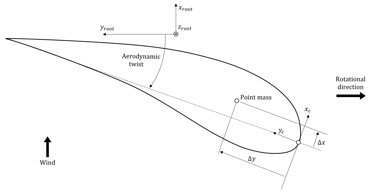
Figure 3: llustration showing the position of point masses relative to the leading edge
Blade lcing
Bladed represents blade ice accretion by adding mass to the blade at the aerofoil leading edge. It is defined in the Blades screen under the Blade Information tab. This additional mass will modify the blade mass totals and mass distribution properties such as Polar mass moment of inertia/unit length and the location of the Mass centre .
There are two available methods for the calculation of ice mass on the turbine blades.
Germanischer Lloyd (GL, 2010) IEC 61400-1 edition 4 standard.
For both ice models, the radial distance from the rotor axis is assumed to be a nominal radius i.e. ignoring the effect of rotor cone, blade prebend and blade root mounting angle. The GL 2010 rotorradius \boldsymbol{R} is always half of the Nominal rotor diameter as shown in the Turbine and Rotor screen found in under the Rotor screen in the Bladed GUl. Each blade station radial position r can be calculated using the blade root length added to the blade station Distance along blade root Z-axis at each blade station.
\textcircled{i} NOTE
The change in mass due to blade icing is not reflected in the Turbine Information screen accessed when clicking the Mass totals... . Instead, the mass distribution and blade mass with ice are provided in the verification file .$vE output when simulations are run.
Ice accretion can also modify the aerodynamic properties of aerofoils. No modification is applied to the aerofoil data that has been input into Bladed. If design standards require these
modifications to be made then it is recommended that the user applies these corrections manually to the aerofoil input data.
GL 2010 Method
The methodology used for the GL 2010 approach is as follows. The mass distribution increases linearly from zero at the rotor axis to the value \mu_{e} at half the radius and then remains constant up the blade tip. The value \mu_{e} is calculated as follows:
\mu_{e}=\,\rho c_{\mathrm{min}}(c_{\mathrm{max}}+c_{\mathrm{min}})(0.00675+\exp\left(-0.32R\right))
where
\boldsymbol{R} is the rotor radius in {\bf m},
c_{\mathrm{max}} is the maximum chord in {\bf m},
c_{\mathrm{min}} is tip chord in m,
\rho is the ice density with default value 700\;\mathrm{kg/m^{3}}
The chord length at the blade tip is an input in Bladed. The maximum chord value is computed using the values from the Blade Geometry information input by the user.
IEC Ed 4 Method
The methodology used for the IEC Ed 4 is to apply a mass distribution that increases linearly from zero at the rotor axis to the maximum value at the blade tip. The ice mass distribution is calculated Using:
M(r)=\rho C_{85}r
where
M(r) is the mass distribution on the leading edge of the rotor blade in {\bf k g}/{\bf m}, \rho is a constant parameter with default value of 0.125\;\mathrm{kg/m^{3}}
C_{85} is the chord length at 85\% rotor radius in m,
_r is the radial position measured from the rotor axis in m.
The parameter C_{85} is calculated by Bladed based on the geometry information input by the user. Last updated 13-12-2024
Blade Local Element Axes System
Consider a blade element with an inboard node A and further outboard node B, as shown in Figure 1. The difference in coordinates between points A and are expressed in the Root Axes coordinates as r_{x},r_{y} and \boldsymbol{r}_{z}, which correspond to the difference in the variables Neutral axis (\mathsf{x}) Neutral axis (y) and Distance along blade root Z axis respectively.To fully define the blade local element coordinate system, two of the three vectors that form the coordinate basis are calculated by Bladed from the user inputs. The element coordinate system is defined as shown in red in the diagram below. The element \times direction vector is known based on the difference in positions of nodes A and B. The local element z direction needs to be calculated to fully define the local element coordinate system for the structural model.
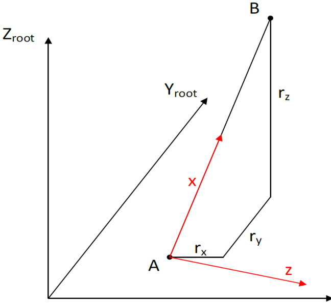
Figure 1: Definition of the blade local element x direction
The element local z-direction vector is calculated by applying 3 successive rotations to the local element z-axis. The 3 rotations are about the blade root axes \mathsf{X},\mathsf{Y} and Z directions. The element local z-axis is assumed initially to be aligned with the X_{r o o t} direction.
Rotation due to principal elastic axes orientation
The first rotation is a rotation about an axis parallel to the Z_{r o o t} axis. The angle of rotation is the Principal elastic axes orientation as specified in the blade inputs screen. This is illustrated in Figure 2.
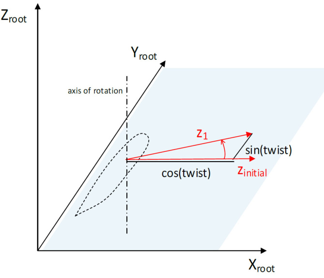
Figure 2: Rotation of local element z direction due to principal elastic axes orientation
Rotation due to prebend
Next,the vector z_{1} is rotated by the prebend angle, by rotating about an axis parall to the Y_{r o o t} axis, as illustrated in Figure 3.
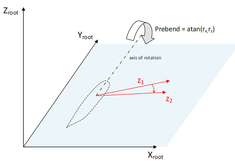
Figure 3: Rotation of blade local element z-axis by prebend angle
Rotation due to sweep
Finally, the vector z_{1} is rotated by the sweep angle, by rotating about an axis parallel to the X_{r o o t} axis, as illustrated in Figure 4.
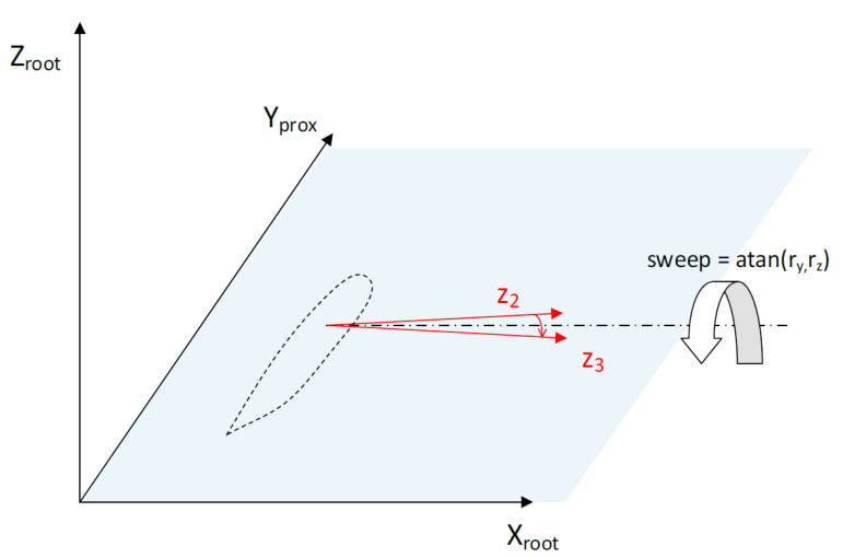
Last updated 13-12-2024
Overview of The Blade Flexibility Options
Bladed utilises a finite element (FE) model to simulate the flexibility of the blades. Additionally, it can incorporate a modal reduction technique to enhance computational efficiency. To account for the non-linear behaviour of larger blades, Bladed offers several geometric stiffness models and supports the definition of multi-part blades.
Users have the option to model the blades in three different ways. These are located in the Flexibility Screen of the GUl and include the following options:
· Finite element (no modal reduction) : This approach involves structural modelling of the blade using finite element analysis without modal reduction.
· Modal reduction : In this method, the blade's structural modelling combines a finite element model with modal reduction.
·Rigid : Disable the Flexibility Enabled option to make the blade completely rigid.
Changing between these three options allows for a convenient way of changing between rigid, modal reduced, or complete finite element blades.
Last updated 13-12-2024
Finite Element Model and Modal Reduction
The structural formulation in Bladed is based on the finite element method (FEM), which is a computational technique used for solving structural dynamics problems. It discretises a structural system into smaller elements, each with specific physical properties (such as density, Young's modulus, shear modulus and so on). These elements are interconnected at discrete points called nodes, forming the overall structural model which is referred to as the flexible body. An illustration of how the blade is discretised into a flexible body can be seen in Figure 1 using a fixed boundary condition. For further details refer to the introduction to flexible components section.
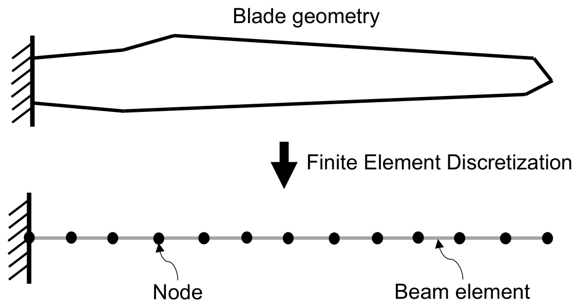
Figure 1: llustration of the blade discretisation into finite elements.
With the basic finite element method the flexible body is described by six degrees of freedom at each node, which means that the complete flexible body will have 6(n-1) degrees of freedom taking into account that the displacement at the proximal node is assumed to vanish (fixed boundary condition). Figure 2 shows the degrees of freedom at each node of a flexible body consisting of a single beam in three dimensions.
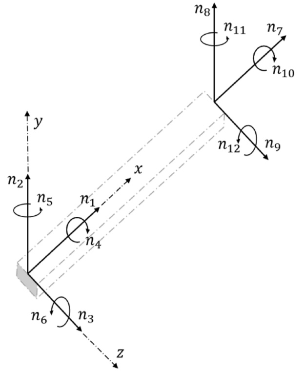
Figure 2: llustration of a beam element with the nodal degrees of freedom.
The flexible body of the blade is based on the structural properties of the blade sections, such as stiffness and mass, which are defined in specific blade section coordinate systems. This will create 6(Sections - 1) degrees of freedom, which can significantly increase the computational effort due to the large number of freedoms involved for long and complex blades. Hence a method to effectively reduce the number of freedoms while still keeping the fidelity and accuracy is preferable and Bladed utilises the method of Modal Reduction.
The user can enable the complete finite element model by using the Finite element (no modal reduction) option found in the Flexibility screen. However, this is not recommended from a calculation speed perspective.
Modal Reduction
An efficient way of increasing the calculation speed is to reduce the number of degrees of freedom that describes the present deformation state of the system by eliminating high frequency modes that do not contribute significantly to the dynamics of the body. This is achieved by expressing the current deformation state in terms of a number of so-called mode shape functions that describe a pre-calculated pattern of the nodal coordinates. This functionality can be switched on by using the Modal reduction option in the Flexibility screen. The number of included mode shapes is determined by the input Number of modes on part , where the "part" refers to the multipart blade definition.
Mode Shapes
The flexible body of the blades can be represented as a finite element model with fixed boundary condition at one end, as depicted in Figure 1. By performing an eigenvalue analysis on this structure, we can compute a set of mode shapes corresponding to the number of degrees of freedom in the model. The eigenvectors of the analysis correspond to the mode shapes which
describe the different vibrational patterns. The resulting eigenvalues correspond to associated frequencies.
The types of mode shapes of a blade are (see Figure 4 for visualisation):
· Flapwise : Refers to the bending of the blade about the Y-axis. Imagine the blade flexing up and down like a flap. This will often be the most flexible degree of freedom with the lowest frequency.
· Edgewise : Involves bending of the blade about the X-axis. Picture the blade bending from side to side. Often stiffer than the flapwise direction.
· Torsional : Occurs when the blade twists around its longitudinal axis (Z-axis). Think of the blade twisting like a corkscrew, changing the angle of attack.
· Axial : It refers to changes along the blade's axial direction (Z-axis). Axial deformation is less commonly discussed in the context of wind turbine blades as it is often a very stiff degree of freedom, having a high frequency and low impact to the overall dynamics.
In the single-part blade model, only normal modes are used. When the multi-part blade model is selected, the inner parts use both normal and attachment modes, while the outermost part uses only normal modes. For further details, please see the normal and attachment modes and blade mode shapes theory sections.
An illustration of the 1st and 2nd edgewise mode shapes can be seen in Figure 3 and different mode shape types can be seen in Figure 4.
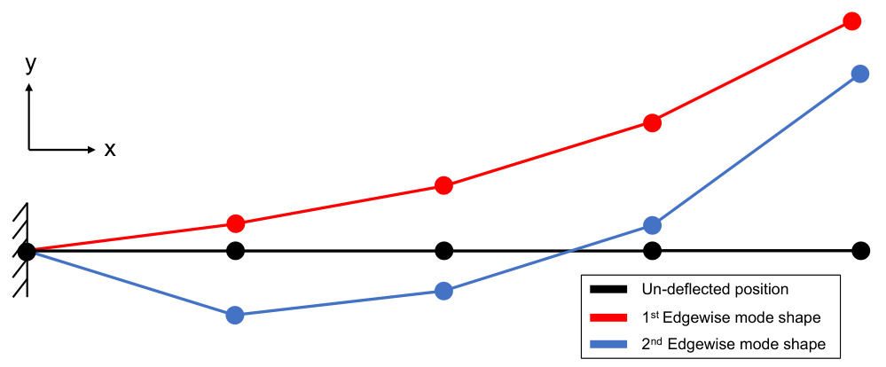
Figure 3: llustration of the 1st and 2nd edgewise mode shapes for a straight blade.
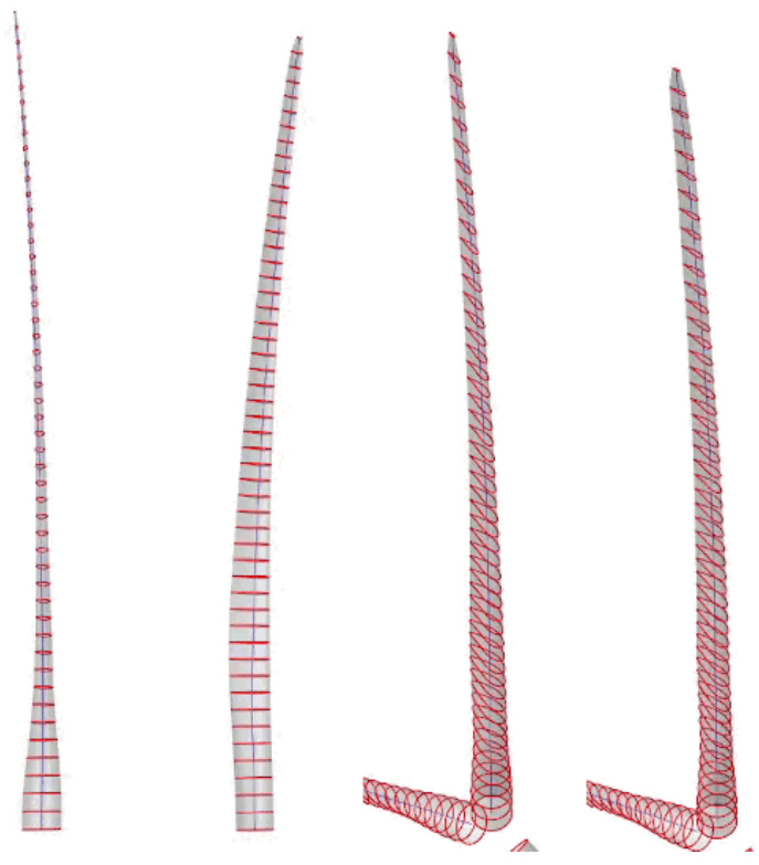
Figure 4: Left to right: Flapwise, edgewise, torsional, axial
Last updated 13-12-2024
Multi-Part Blades
The simplest approach used in Bladed to model the blade flexibility is to model the blade as a single linear finite element body. Several linear mode shapes that include deflections of the wholeblade are calculated to account for blade deflection. This is illustrated in Figure 1.
Single flapwise mode
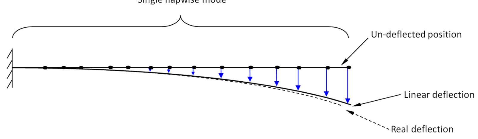
Figure 1: Linear single part blade
Using whole-blade linear modes results in fast simulations as the number of degrees of freedom to model the blade deflections is small, and the freedom frequencies are relatively low. This approach often gives an accurate representation of blade dynamics. However, for this approach to be valid, the deflections of the blade must be small. Many modern blade designs are very flexible, meaning that the small deflection assumption in the linear model become invalid. This can lead to inaccuracies in predicting the blade dynamic response, in particular the blade torsion.
One method to maintain the small angle assumption for the blade modes is to split the blade into several linear parts. Figure 2 shows a schematic of modelling a blade using two linear parts.
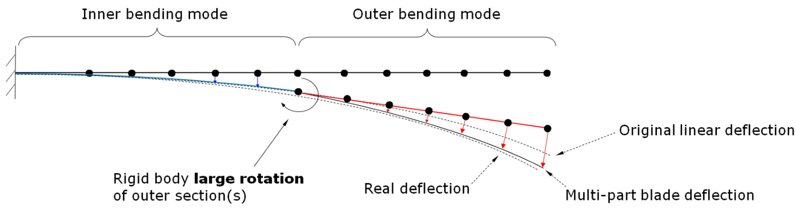
Figure 2: Non-linear wind turbine blade model using two linear parts
The outer blade part can undergo a rigid body rotation based on the deflection and rotation of the inner part, as well as including linear mode deflections. The deflections within each linear part are therefore smaller than if using a single linear blade part. Splitting the blade into several parts allows for non-linear load transfer between each linear part, and a more accurate model of the blade deflection.
Specifying Blade Parts
The user needs to specify the boundaries of the parts in the blade. This is done in the Flexibility SCreen within the BladePartModalModeller,where the First station and Last station are required inputs. An illustration of a blade with 3 parts can be seen in Figure 3.
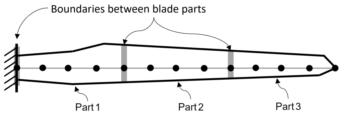
Figure 3: llustration of blade with 3 parts and boundaries
The number of included modes per part is specified using Number of modes on part property which is available for each added part. The user needs to carefully validate the included wholeblade modes and consider whether it includes the wanted dynamic responses such as torsional or flapwise modes etc.
For maximum accuracy, enough blade parts should be specified to ensure that deflections remain small within each blade part. When performing convergence tests for multi-part blade models, it is recommended to run some time domain tests with the maximum number of blade parts in order to establish a baseline converged dynamic response.
\textcircled{i} NOTE
For blades with more than one part, it is recommended to use the implicit Newmark- \cdot\upbeta integrator to improve simulation speed while retaining accurate solutions.
Note on Damping and Multi-Part Blades
The user must specify whole-blade modes even when using multi-part blades, as Bladed will calculate the appropriate damping ratios for the individual blade parts based on the specified whole-blade damping. This is also valid for Finite element (no modal reduction) models, as Bladed will convert the whole-blade shapes into finite element degrees of freedom. Explained in further details below.
When a blade is split into several linear parts, mode shapes (or finite element degrees of freedom) are calculated for each linear part. In the Bladed modal structural dynamics formulation, modal damping must be specified for each mode on each blade part. However, in general the damping value for these individual modes would not be known by the blade designer, as these modes for the individual blade parts cannot be observed individually in reality to measure their damping.
To overcome this difficulty, Bladed calculates whole-blade modes for the multi-part blade by solving the Eigenvalue solution for all of the blade parts together. The whole-blade modes are made up of contributions from the individual blade part modes. The whole-blade modes should have very similar shapes and frequencies to the usual whole-blade mode shapes found for a linear blade model, if enough modes have been specified on each part. Damping ratios can then be specified for the whole-blade blade modes, and Bladed will calculate the appropriate damping ratios for the individual blade parts.
The number of whole-blade modes for the blade is equal to the total number of modes on all of the blade parts. For example, for a blade split into 4 parts with 8 modes on each part, there are 32 whole-blademodes.
Last updated 13-12-2024
Geometric Stiffness Models
Geometric stiffening models account for changes in structural response due to structural deflection from the reference (undeflected) state. Bladed provides models that include contributions from element axial and shear internal forces. They can be selected in the Flexibility SCreen under the Simulation flexibility settings -> Blade geometric stiffness model.
There are two geometric stiffness settings available for the blades:
Axial loads only : The effect of internal forces along the element axis on dynamic response is included. This primarily accounts for "centrifugal stiffening" in the blade dynamic response. Geometric stiffness axial and shear forces are included when calculating the internal member loads. See Geometric stiffness due to element axial forces for more details. ·Full model with orientation correction : The effect of internal axial and shear forces on dynamic response is included. This model can enhance the prediction of torsion deflection in the blade. This model should be used with caution as it is only accurate when deflections within each blade part remain small (less than \mathord{\sim}5\mathord{-}7 degrees). If several blade parts are used then this model can be activated to improve the accuracy of the solution, and will allow use of fewer blade parts than when using the AxialLoadsonly model. See Geometric stiffness due to element shear forces for more details.
When evaluating the geometric stiffness effect of shear forces, it is crucial to consider to account for the change in orientation of the torsion axis of the blade elements due to deflection.
Last updated 13-12-2024
Whole-Blade Damping
Bladed is able to introduce modal damping by applying a damping ratio for each whole-blade mode. The user can choose how many whole-blade modes to specify damping ratios for using the Modes with damping defined variable in the Whole-blade modes found in the Flexibility screen. Any higher frequency modes will be assigned frequency proportional damping, based on the damping of the highest mode with damping defined. This approach applies high damping to high frequency modes and effectively excludes the higher whole-blade modes from the blade dynamic response, so that they do not cause erroneous instability. See the theory section description of blade damping for more details. Note that Bladed will then automatically calculate the damping values to assign to each individual blade part (see multi-part blade definition).
<html>| Modal analysis results and damping inputs | |||||||
| Whole-blade modes | Tower modes | ||||||
| View blade mode | |||||||
| Modes with damping defined 10 | |||||||
| ID | Damping Ratio (%) | Name | Modal Frequency (Hz) | ||||
| 0.491 | 1st flapwise normal mode | 0.3851219 | |||||
| 2 | 0.507 | 1st edgewise normal mode | 0.5186781 | ||||
| 3 | 1.336 | 2nd flapwise normal mode | 1.059886 | ||||
| 4 | 1.364 | 2nd edgewise normal mode | 1.487568 | ||||
| 5 | 2.749 | 3rd flapwise normal mode | 2.21401 | ||||
| 6 | 2.857 | 3rd edgewise normal mode | 3.203897 | ||||
| 7 | 3.555 | 4th flapwise normal mode | 3.676734 | ||||
| 8 | 1.896 | 5th flapwise normal mode | 3.980007 | ||||
| 9 | 5.689 | 6th flapwise normal mode | 5.300175 | ||||
| 10 | 5.109 | 7th flapwise normal mode | 5.769784 | ||||
| 11 | Frequency proportionall | 1st torsional normal mode | 6.413283 | ||||
| 12 | Frequency proportional | 8th flapwise normal mode | 7.315367 | ||||
| 13 | Frequency proportional | 4th edgewise normal mode | 8.718863 | ||||
| 14 | Frequency proportional | 9th flapwise normal mode | 9.455891 | ||||
| 15 | Frequency proportional | 10th flapwise normal mode | 9.527341 | ||||
| 16 | Frequency proportional | 11th flapwise normal mode | 11.50475 | ||||
| 17 | Frequency proportional | 5th edgewise normal mode | 12.21184 | ||||
Figure 1: Example of whole-blade modes screen for specifying damping ratios for each mode Last updated 13-12-2024
Output of Blade Loads
View available Blade outputs ,as seen in Figure 1, by clicking the Calculation Outputs... button on the Calculations screen. The outputs must be for either the First blade, All blades , or not at all( None ). The output settings defined here do not affect the Aerodynamic Information , Performance Coefficients and Steady Power Curve calculations, as they produce a pre-defined set of outputs. A customised blade load output file can also be created and is described in the section on Load Configuration File.
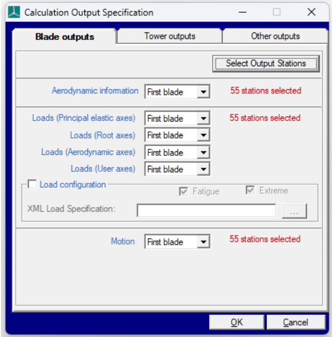
Figure 1: Calculation Output Specification screen for Blade Outputs
Read more about the coordinate systems where the loads outputs are available in the following links:
Principal elastic axes Root axes
Aerodynamic axes User axes
For each of the output categories in the Blade outputs ,the information may be generated at any or all of the blade stations. Click Select Output Stations to determine which information is required at which stations. Click Add to define additional points where interpolated loads will be Output.
<html>| Blade Outputs | |||||||
| Distance along blade, m | Blade station number | Aero data? | Blade loads? | Blade motion? | |||
| 0 | Yes | Yes | Yes | ||||
| 2.756 | 2 | Yes | Yes | Yes | |||
| 4.1343 | 3 | Yes | Yes | Yes | |||
| 5.51253 | 4 | Yes | Yes | Yes | |||
| 6.89437 | 5 | Yes | Yes | Yes | |||
| 9.65766 | 6 | Yes | Yes | Yes | |||
| 12.4153 | 7 | Yes | Yes | Yes | |||
| 15.1714 | 8 | Yes | Yes | Yes | |||
| 17.9279 | 9 | Yes | Yes | Yes | |||
| 20.6845 | 10 | Yes | Yes | Yes | |||
| 23.441 | 11 | Yes | Yes | Yes | |||
| 26.1973 | 12 | Yes | Yes | Yes | |||
| 28.9534 | 13 | Yes | Yes | Yes | |||
| PP | |||||||
| OK | Cancel | ||||||
It is important to note that the principal elastic axes and root axes stations coincide with the underlying finite beam element model nodes. The root axes coordinates have the same origin rotated to align with the blade root. The aerodynamic and user axes potentially have origins that do not coincide with the underlying finite element beam model nodes. These load outputs are found by transforming the finite element loads (in the principal elastic axes coordinates) to the aerodynamic or user axis coordinate centre. The transformation accounts for additional M_{x} and M_{y} bending moments that are generated at the aerodynamic or user axis centre by the element axial force F_{z} in the principal elastic axes system, due to the offset in the aerofoil plane between these two coordinate centres. This effectively estimates the load that would have occurred if the load was carried through an axis at the aerodynamic axis or user axis centre. There is some approximation in this method as the aerodynamic and user axis loads are not the true load path. Any changes to the blade dynamics (e.g. deflections or loads) that might result from such a change in load path are not accounted for.
An additional set of blade root loads, using a coordinate system fixed to the blade root in the hub (i.e., inboard of the pitch bearing), is output as part of the Hub loads (Rotating frame) output group found in Other outputs , as seen in Figure 1. For more details on this coordinate system, refer to the article on Rotating Hub Loads.
Load Configuration File
A blade manufacturer may specify a customised blade load output format, for a particular blade, in an XML format load configuration file. Customised blade load output files can then be generated, from a dynamic simulation, by selecting the Load configuration checkbox and specifying the load configuration file in the XML Load specification field on the Blade Outputs tab of the Calculation Output Specification window, as shown below (this window can be opened using the Calculation Outputs.. button on the Calculations window, or the Outputs.. Option of the Specify menu.).
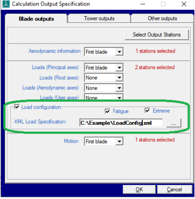
Figure 4: Blade load configuration file
If the Extreme checkbox is also selected, customised extreme blade loads will be written to an output file with .blc filename extension. Extreme load output files can be generated for each blade using the Additional Items option of the Specify menu and selecting Output individual blade extreme loads .
Last updated 13-12-2024
Blade Loads Outputs at Principal Elastic Axes System
· The positive z-axis follows the local deflected neutral axis at each blade station towards the blade tip. · The positive y-axis is defined by the principal elastic axes orientation. · The positive x-axis is orthogonal to the y and z and follows the right-hand rule.

Figure 1: Blade principal elastic axes coordinate system
Note that there is a subtle difference between the principal elastic axes coordinate system and the underlying blade local element axes coordinate system, whereas the latter is used to calculate the orientation of the principal elastic axes. The Principal elastic axes orientation is calculated by taking the average orientation of the two blade elements at the node where the elements join. This is illustrated in Figure 2. The two adjoining local element frames are shown in green and red. The principal elastic axes output frame is shown in blue.
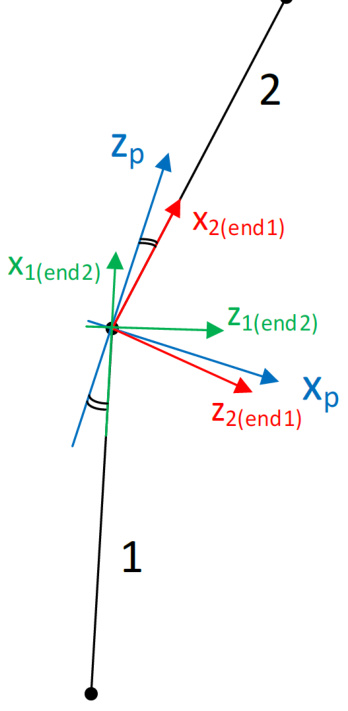
Figure 2: Principal elastic axes and local element axes orientations
Last updated 13-12-2024
Blade Loads Outputs at Root Axes System
The body-fixed coordinate system of the blade is the root axes coordinate system. The blade root coordinate system serves as the reference frame for defining the blade's geometry. The orientation of the axes is fixed to the blade root and does not rotate with either twist or blade deflection. The axis set does rotate about the z axis with pitch. For output loads, the origin of the axes is on the neutral axis at each local deflected blade station.
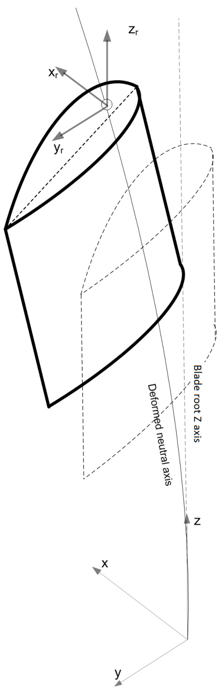
Figure 1: Blade root axes coordinate system
Last updated 13-12-2024
Blade Loads Outputs at Aerodynamic Axes System
· The x-axis is perpendicular to the local aerodynamic chord line.
· The positive y-axis is aligned along the local aerodynamic chord line from the leading edge to the trailing edge.
· The z-axis is parallel to the local deflected neutral axis at each blade station and increases towards the blade tip.
For output loads, the origin of the axes is on the chord line at 25\% chord from the leading edge at each local deflected blade station. In Figure 1 the y_{r} -component points towards the trailing edge of the airfoil. However, for anti-clockwise configurations the y_{r} -component points towards the leading edge as the airfoil is rotated. Thus the orientation of the aerodynamic axes does not change between clockwise and anti-clockwise rotors.
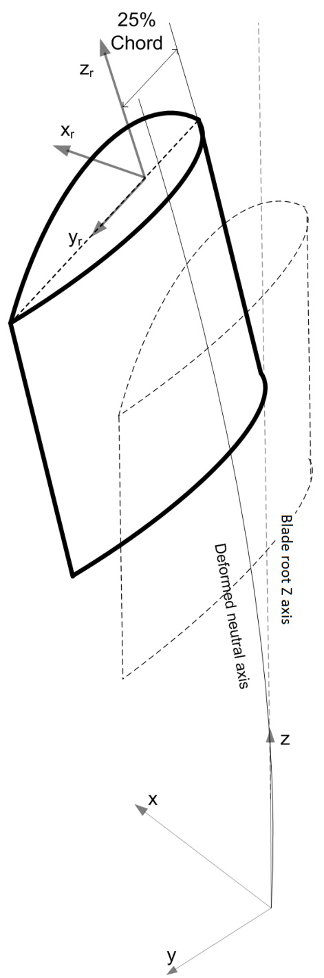
Figure 1: Blade aerodynamic axes coordinate system
Blade Loads Outputs at User Axes System
The user axes system is a custom coordinate system that can be defined by the user for outputting blade loads. It is defined in the Blades screen in the Blade Geometry tab. At the bottom of the screen it is possible to define the user defined axis directions for the z-axis and y-axis. The y-axis can follow either the untwisted root y-axis, principal elastic y-axis or the aerodynamic twist. The zaxis options and their implications are explained below.
User axes: Z-axis follows neutral axis or root z-axis
The origin of the axes is specified as percentages of chord, parallel and perpendicular to the chord at each blade station as shown in Figure 1. The user can specify whether the z-axis is parallel to the root axis or the local neutral axis. Similarly, the user can independently specify whether the y-axis is aligned to the principal elastic axes orientation, the aerodynamic twist, or the root axis.
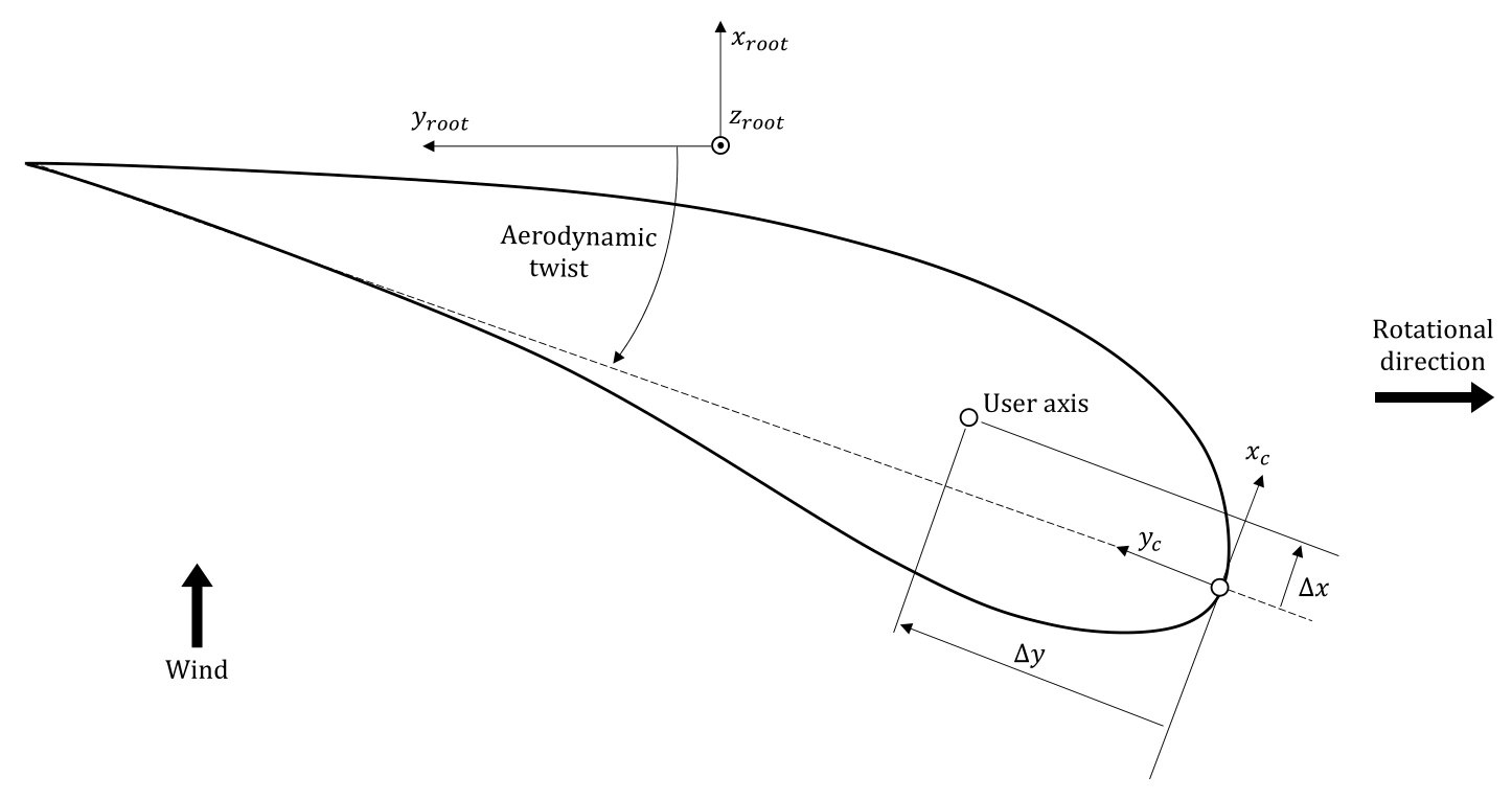
Figure 1: Position of the user defined output axis
User axes: Z-axis follows user axis
This option enables the user to create a new custom output coordinate system. This system is defined relative to the local element coordinate system that is illustrated in Figure 2. A planar view of a simple blade comprising indexed blade stations with adjoining elements is provided. In this example, only prebend of the neutral and user axes is considered. Presweep, principal elastic axes orientation and aerodynamic twist are zero. The inboard station number near the blade root is 1 and the most outboard near the blade tip is 3. At each station, the position of the neutral axis node is provided by the user. The consecutive neutral axis nodes are connected via piecewise linear "elements" in order of ascending numerical station index.
The blade element coordinate system is denoted by the subscript e. For the nth piecewise linear element at node m, the x_{e_{n,m}} -axis runs parallel to the line adjoining consecutive neutral axis nodes. Positive direction is from the blade root to tip. The y_{e_{n,m}} -axis and z_{e_{n,m}} -axis are determined by the principal elastic axes orientation around the x_{e_{n,m}} -axis. The principal elastic axes orientation is specified by the user and per node. Hence, the direction of the y_{e_{n,m}} -axis depends on both the element and the node index. When the principal elastic axes orientation is zero z_{e_{n,m}} lies in the x_{r}, z_{r} root axes plane.
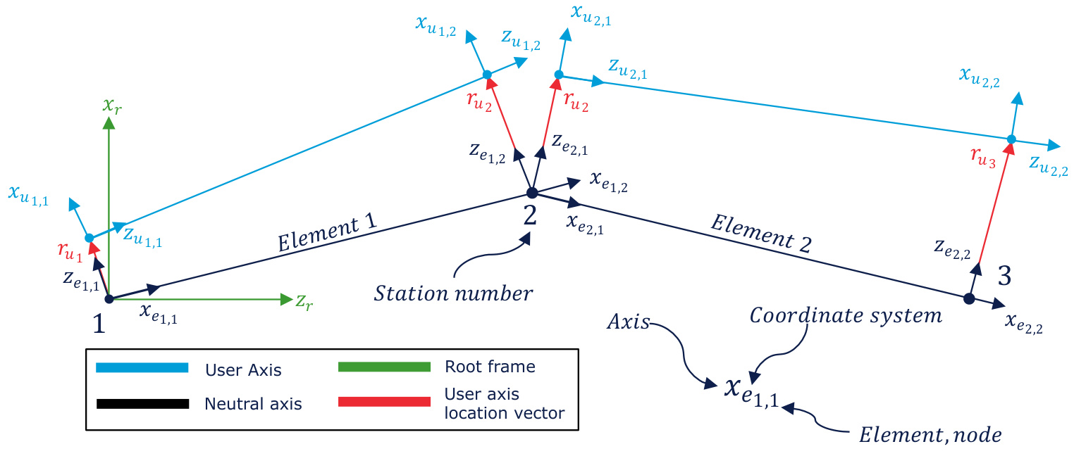
Figure 2: Definition of the user axis location and orientation when z-axis follows user axis
Figure 3 illustrates a blade station and presents key geometric information necessary to understand the user axes coordinate system. The diagram is now drawn assuming a straight neutral axis (no blade prebend or presweep) in the spanwise direction. Also, the aerodynamic twist and principal elastic axis orientation are considered non-zero. In this simple case the various properties such as principal elastic axis orientation and aerodynamic twist along with user axis position are defined in the root axes plane denoted x_{r},y_{r}
The user axis coordinate systems are derived from the element frame. More generally, the user axis inputs x^{\prime},y^{\prime} are defined by the user using the chord coordinate system. These are rotated and translated into the local element coordinate system creating the \boldsymbol{r}_{u_{m}} vector as shown in Figure 3. The \boldsymbol{r}_{u_{m}} vector lies in the y_{e_{n,m}}\mathrm{~,~}z_{e_{n,m}} plane.
Figure 2 demonstrates that for intermediate nodes the same \boldsymbol{r}_{u_{m}} vector is applied to the adjoining node for both the inbound and the outbound element as illustrated by the \boldsymbol{r}_{u_{2}} vector. For each element, \boldsymbol{r}_{u_{m}} vectors are added to the pair of neutral axis nodes to create two points that lie on the user axis. The z_{u_{n,m}} -axis is parallel to the line connecting these points as illustrated in Figure 2. Figure 2 also demonstrates that the user axis is discontinuous between adjoining blade stations. It is assumed that the variation of the neutral axis orientation between blade stations is small resulting in the discontinuities being smal/neglible. Finally, igure 2 also shows that the \boldsymbol{x}_{u_{n,m}} axis lies in the x_{r},z_{r} plane.
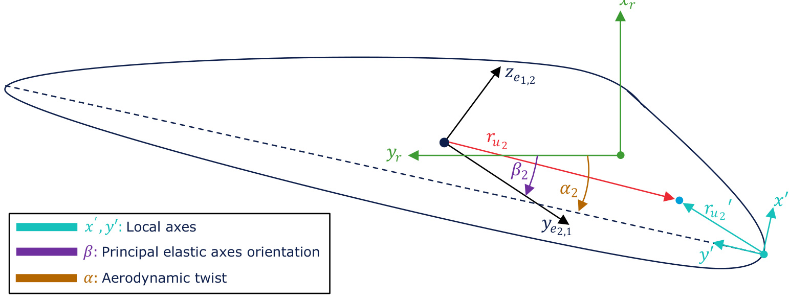
Figure 3: Local aerofoil cross section at station 2 showing x^{\prime},y^{\prime} coordinate system.
Figure 4 provides an overview of the user axis in the more general case where the user specifies a blade with prebend and presweep, where the aerodynamic twist \& principal elastic axis orientation are non-zero and the user axis values are also non-zero. The direction of the y_{u_{n,m}} -axis is determined by a rotation around the z_{u_{n,m}} -axis of either the aerodynamic twist (if y-axis follows aerodynamic twist is selected) or zero twist(if y-axis follows untwisted root axis is selected) as shown in Figure 4. Note that the aerodynamic twist and principal elastic axes orientation inputs are defined as positive clockwise rotations. The direction of the \boldsymbol{x}_{u_{n,m}} -axis is the cross product of the y_{u_{n,m}} -axis and z_{u_{n,m}} -axis. This defines a right-handed coordinate system.
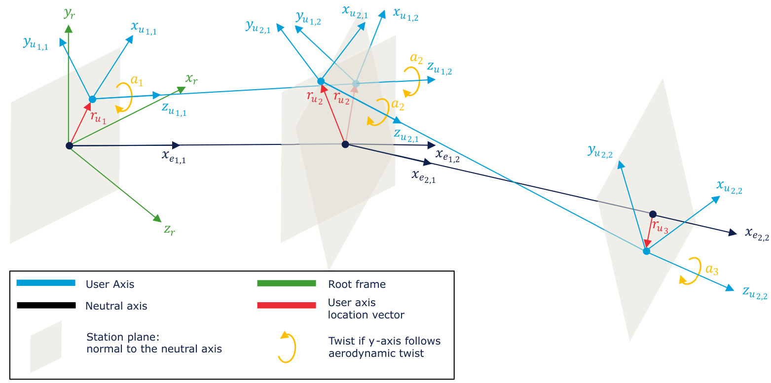
Figure 4: User axis illustrated in three dimensions show the twist
To compute the user axis load output the moments from the element coordinate system must be translated and rotated into the user axis frame. Note that the user axis potentially does not coincide with the blade element axis. An additional moment is added/subtracted at each station to accountforthis:
M_{u}=R_{e u}\left(M_{e}-r_{u_{1}}\times F_{e}\right)
As the relative translation \boldsymbol{r}_{u_{m}} and rotation R_{e u} between the user axis and the associated element coordinate system are independent of blade deflection, the same values at each blade station are used for the entire time domain simulation. Table 2 lists the coordinate system and location used at each station. The first station reports the loads in the outboard user axis \boldsymbol{u}_{1,1} coordinate system and for the remainder of the stations, the inboard user axis _{u_{x,2}} coordinate system is used.
Table 2: Load output for each station in Figure 2 and Figure 4
<html>| Station | User AxisCoordinateSystem | Offset |
| 1 | U1,1 | ru1 |
| 2 | U1,2 | |
| 3 | U2,2 | u3 |
The location of the user axis points in the root coordinate system at the undeflected reference position can be evaluated in the verification file ( \nleq\lor\in 一
The combination of both the z-axis follows user axis and y-axis follows principal elastic axes is not supported.
Last updated 13-12-2024
Output of Blade Kinematics Blade Deflection Outputs
Blade deflections can be output at any station along the blade by activating Motion found in the Blade outputs ,as seen in Figure 1, by clicking the Calculation Outputs... button on the Calculations screen. The outputs must be for either the First blade , All blades , or not at all (None ).
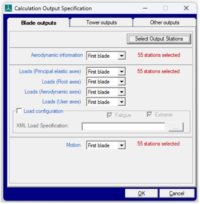
Figure 1: Calculation Output Specification screen for Blade Outputs
Blade deflections are given relative to the blade root coordinate system, with or without the pitch.
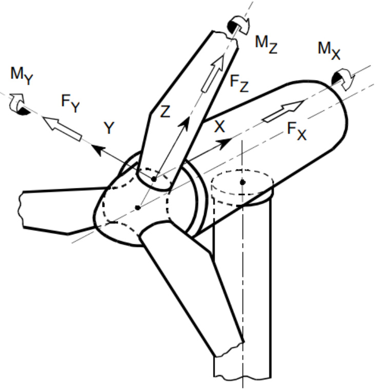
Figure 2: Blade root coordinate system, illustrated for zero cone and pitch.
Blade Acceleration Outputs
Blade accelerations can be output adding the following code to Project Info:
MSTART EXTRA OutputBladeAcc 1 MEND
Accelerations will be output at the same stations as the blade deflections. Accelerations are output in the blade principal elastic axes coordinates.
Blade Strain Gauge Outputs
The external controller is already provided with a set of loading data, but it is possible to add additional strain gauges at any station on the tower or blade. Although called "strain gauges", these actually report forces and moments. Once specified, these will be updated before each call to the discrete external controller. Strain gauges on the blades are defined with a distance with the following code in Project Info:
MSTARTEXTRA
NUMSGAUGES * number of blade strain gauge definitions to follow
SGDIST * Distance along the blade
MEND
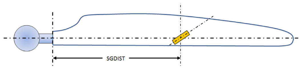
Figure 3: Blade strain gauge position specification
The resulting load can be retrieved in the external controller using the function GetMeasuredBladeStrainGaugeFx , changing the last two letters for the relevant load component.
Blade Accelerometers Outputs
There are already a number of locations where the accelerations are measured on each discrete controller time-step. Additional locations can be added to the blades in a similar manner as for strain gauges. Accelerometers on the blades are defined in a similar manner to strain gauges with the following code in Project Info:
MSTART EXTRA
NUMBLADEACCELEROMETERS ^* The number of blade accelerometer definitions that will follow. ACCDIST * Distance along the blade from blade root. This line is repeated for each accelerometer definition
MFNIn
The resulting accelerations are provided for X, Y, Z in the local blade's coordinates.