obsidian_backup/力学书籍/FASTLoads/auto/FASTLoads.md

The following are derivations of the output loads available in FAST for a 2-bladed turbine configuration. The loads for a 3-bladed turbine are very similar. Note that some of the loads are given multiple names in order to support variation among the user’s preferences.

Along with most of the loads are associated partial loads. These partial loads will be used at the end of this document to redevelop portions of the equations of motion to speed up the computations. The definition of these partial loads is as follows:

F_{_{S o u r c e}}^{X_{i}}\left(\ddot{q},\dot{q},q,t\right)\!=\!\!\left(\sum_{r=I}^{22}F_{S o u r c e_{r}}^{X_{i}}\left(q,t\right)\ddot{q}_{r}\right)\!\!+\!F_{_{S o u r c e_{t}}}^{X_{i}}\left(\dot{q},q,t\right)

where FSXoiur are the partial forces and F_{S o u r c e_{t}}^{X_{i}} is all components of F_{S o u r c e}^{X_{i}} that are not of this form.

M_{S o u r c e}^{N_{i}@X_{i}}\left(\ddot{q},\dot{q},q,t\right)\!=\!\!\left(\sum_{r=I}^{22}{M_{S o u r c e_{r}}^{N_{i}@X_{i}}\left(q,t\right)\ddot{q}_{r}}\right)\!+\!{M_{S o u r c e_{t}}^{N_{i}@X_{i}}\left(\dot{q},q,t\right)}

where MSNoi u@rcXei are the partial moments and M_{S o u r c e_{t}}^{N_{i}(\omega X_{i}} is all components of M_{S o u r c e}^{N_{i}(\varpi X_{i}} that are not of this form.

To find the loads characterizing the constraint forces between two bodies, say A and B, all that is needed is to remove body B from the equations of motion and determine what equivalent load applied on A would give the same effect that body B had on A originally.

Blade 1 Root Loads:

There are 10 output loads at the root of blade 1. 5 of them are the 3 components of the root force F_{B I}^{s t}(\boldsymbol{O}) (2 components are expressed in both the coned and blade reference frames). The other 5 are the 3 components of the root bending moments, M_{B I}^{H}({\boldsymbol{O}}) (again, 2 components are expressed in both the coned and blade reference frames). If blade 1 is to be removed from the turbine, loads F_{B I}^{s t}(\boldsymbol{O}) and M_{B I}^{H}({\boldsymbol{O}}) applied to the hub at the blade 1 root (r=0) must give the equivalent effect of blade 1 in the resulting equations of motion. The new generalized active force for the equations of motion resulting from these new loads is:

\begin{array}{r l}{F_{r}\big|_{B I}={^{E}\pmb{\nu}_{r}^{C}\cdot^{C}\cdot^{C}\pmb{F}_{B I}^{C}}+{^{E}\pmb{\omega}_{r}^{H}\cdot^{M}\pmb{{\cal H}}_{B I}^{H}}}&{{}\left(r=I,2,\ldots,22\right)}\end{array}

where the equivalent loads acting at the hub’s center of mass (point C) are related to F_{B I}^{s t}(\boldsymbol{O}) and M_{B I}^{H}({\boldsymbol{O}}) because the hub is rigid as follows:

FBC1=FBS11 (\!\!\!\begin{array}{c c c c c c c c c}{{(\!\!0)}}&{{\mathrm{and}}}&{{}}&{{M_{B I}^{\!\scriptscriptstyle H}=M_{B I}^{\!\scriptscriptstyle H}(\!\!0)+r^{c s I}(\!\!0)\times F_{B I}^{s\!\scriptscriptstyle I}(\!\!0)}}&{{\mathrm{or}}}&{{}}&{{M_{B I}^{\!\scriptscriptstyle H}=M_{B I}^{\!\scriptscriptstyle H}\left(\!\!0\right)+\left[r^{Q s I}\left(\!\!0\right)+\frac{1}{2}r^{Q s}\left(\!\!0\right)\right]^{\!\!\scriptscriptstyle T}.}}\end{array} −rQC×FBS11(0 )

But since {}^{E}{\pmb{\nu}}_{r}^{c}={}^{E}{\pmb{\nu}}_{r}^{Q}+{}^{E}{\pmb{\omega}}_{r}^{H}\times{\pmb{r}}^{Q C} , this generalized active force can be expanded to:

Fr B1=(E \begin{array}{r l}{\mathbf{\nabla}_{r}^{\rho}+^{E}\boldsymbol{\omega}_{r}^{H}\times\mathbf{\boldsymbol{r}}^{Q C}\Big)\cdot F_{B I}^{S I}\left(\theta\right)+^{E}\boldsymbol{\omega}_{r}^{H}\cdot\left\{{M}_{B I}^{H}\left(\theta\right)+\left[{\boldsymbol{r}}^{Q S I}\left(\theta\right)-{\boldsymbol{r}}^{Q C}\right]\times{F}_{B I}^{S I}\left(\theta\right)\right\}}&{\left(r=I,2,\ldots,K\right)^{T},}\end{array} 22)

Now applying the cyclic permutation law of the scalar triple product:

=^{E}\nu_{r}^{Q}\cdot F_{B I}^{S I}\left(\theta\right)+^{E}\omega_{r}^{H}\cdot\left\{r^{Q C}\times F_{B I}^{S I}\left(\theta\right)\right\}+^{E}\omega_{r}^{H}\cdot\left\{M_{B I}^{H}\left(\theta\right)+\left[r^{Q S I}\left(\theta\right)-r^{Q C}\right]\times F_{B I}^{S I}\left(\theta\right)\right\}+^{E}\omega_{r}^{H}\cdot\left[M_{B I}^{H}\left(\theta\right)+\left[r^{Q S I}\left(\theta\right)-r^{Q C}\right]\times F_{B I}^{S I}\left(\theta\right)\right\}

which simplifies to:

F_{r}\Big|_{B I}=^{E}\nu_{r}^{Q}\cdot F_{B I}^{S I}\left(0\right)+^{E}\omega_{r}^{H}\cdot\Big[M_{B I}^{H}\left(0\right)+r^{Q S I}\left(0\right)\times F_{B I}^{S I}\left(0\right)\Big]\;\;\;\left(r=I,2,\ldots,22\right)

[This can also be simplified to F_{r}\big|_{B I}={}^{E}\nu_{r}^{S I}\left(0\right)\cdot F_{B I}^{S I}\left(0\right)+{}^{E}\omega_{r}^{H}\cdot M_{B I}^{H}\left(0\right)\quad\left(r=I,2,...,22\right) , which will be used later in the ensuing analysis.]

This generalized active force must produce the same effects as the generalized active and inertia forces associated with blade 1. Thus,

F_{r}\big|_{B I}=F_{r}^{*}\big|_{B I}+F_{r}\big|_{A e r o B I}+F_{r}\big|_{G r a v B I}+F_{r}\big|_{E l a s t i c B I}+F_{r}\big|_{D a m p B I}\quad\big(r=I,2,\dots,22\big)

Since {}^{E}{\nu}_{r}^{c} and ^E{\omega}_{r}^{H} (and ^E_{\nu_{r}^{Q}} and ^E_{\pmb{\nu}_{r}^{S I}}({\cal O})) are equal to zero unless r=1,\!2 ,…,14;Teet, the generalized active forces associated blade elasticity and damping do not contribute to the root loads (since also, F_{r}\big|_{E l a s t i c B I} and F_{r}|_{D a m p B I} are equal to zero within this range of r\,\mathbf{\dot{s}} ). So,

\left.F_{r}\right|_{B I}=F_{r}^{*}\Big|_{B I}+F_{r}\Big|_{A e r o B I}+F_{r}\Big|_{G r a v B I}\quad\left(r=I,2,...,I\mathcal{I};T e e t\right)

Thus,

Fr B1= \begin{array}{l}{{\displaystyle\int_{0}^{B I d F l e c L}\varepsilon_{\nu_{r}^{S I}}(r)\cdot\left[F_{A e r o B I}^{S I}\left(r\right)-\mu^{B I}\left(r\right)g\varepsilon_{2}-\mu^{B I}\left(r\right)\varepsilon_{a}^{\phantom{S I I}}\varepsilon_{\phantom{S I I}}^{\phantom{S I I}}\left(r\right)\right]d r+\lefteqn{\displaystyle\int_{0}^{B I d F l e c L}\varepsilon_{\omega_{r}^{M I}}^{{M I}}\left(r\right)\cdot M_{A e r o B I}^{M I}\left(r\right)}=}}\\ {{\displaystyle+\,^{E}\nu_{r}^{S I}\left(B I d F l e x L\right)\cdot\left\{F_{T p D r a g B I}^{S I}\left(B I d F l e x L\right)-m^{B I T i p}\left[g z_{2}+\varepsilon_{a}^{\phantom{S I I}}\left(B I d F l e x L\right)\right]\right\}}}\end{array} oB1(r ) dr (r=1,2,,14;Teet)

^{E}\nu_{r}^{s l}(r){=}^{E}\nu_{r}^{g}{+}^{H}\nu_{r}^{s l}(r){+}^{E}\omega_{r}^{H}\times{r}^{g s l}(r)

Fr \begin{array}{c}{{\biggl|_{B I}=\displaystyle\int\displaystyle\sum_{\theta}^{B I d F e x t}\left[^{E}\nu_{\nu}^{Q}+^{H}\nu_{\nu}^{S I}\left(r\right)\right]\cdot\left[F_{A e r o B I}^{S I}\left(r\right)-\mu^{B I}\left(r\right)g z_{2}-\mu^{B I}\left(r\right)^{E}a^{S I}\left(r\right)\right]d r}}\\ {{+\left[^{E}\nu_{\nu}^{Q}+^{H}\nu_{r}^{S I}\left(B I d F l e x L\right)\right]\cdot\left\{F_{T i p D r a g B I}^{S I}\left(B I d F l e x L\right)-m^{B I T i p}\left[g z_{2}+^{E}a^{S I}\left(B I d F l e x L\right)\right]-m^{B I d F i c e n t}\right.}}\\ {{+\left.\displaystyle\int\displaystyle\sum_{\theta}^{B I d F e x L}\left[^{E}\omega_{r}^{H}\times r^{Q S I}\left(r\right)\right]\cdot\left[F_{A e r o B I}^{S I}\left(r\right)-\mu^{B I}\left(r\right)g z_{2}-\mu^{B I}\left(r\right)^{E}a^{S I}\left(r\right)\right]d r+\displaystyle\int\displaylimits_{0}^{B I d F i c e n t}}}\\ {{+\left[^{E}\omega_{r}^{H}\times r^{Q S I}\left(B I d F l e x L\right)\right]\cdot\left\{F_{T i p D r a g B I}^{S I}\left(B I d F l e x L\right)-m^{B I T i p}\left[g z_{2}+^{E}a^{S I}\left(B I d F l e x L\right)\right]\right\}.}}\end{array} L)} (r=1,2,,14;Teet) EωrM1(r )⋅MAMe1roB1(r ) dr L)}

However, since r is constrained to be between 1,2,…,14;Teet and since {}^{H}\nu_{r}^{s t}(r) is equal to zero and ^{E}\pmb{\omega}_{r}^{M I}\left(r\right) equals ^E\pmb{\omega}_{r}^{H} with this constraint, this can be simplified as follows:

\begin{array}{c}{{\cdot\rfloor_{B I}=\displaystyle\int_{0}^{B I F l e c L}\varepsilon_{\nu_{r}^{Q}}\cdot\left[F_{_{A e r o B I}}^{S I}\left(r\right)-\mu^{B I}\left(r\right)g z_{2}-\mu^{B I}\left(r\right)\varepsilon_{a}^{S}a^{S I}\left(r\right)\right]d r+}}\\ {{\overset{B I d F e c L}{{+}}}}\\ {{+}}\\ {{\overset{B}{\lefteqnrightarrow}}}\\ {{+\left[\begin{array}{c}{{\displaystyle E\,\omega_{r}^{H}\times r^{Q S I}\left(r\right)-\left[F_{A e r o B I}^{S I}\left(r\right)-\mu^{B I}\left(r\right)-\mu^{B I}\left(r\right)g z_{2}-\mu^{B I}\left(r\right)^{E}a^{S I}\left(r\right)\right]d r+\displaystyle\int_{0}^{B I d F l e c s}\int_{0}^{1}\left(r\right)^{2}\left(r\right)^{2}\varepsilon_{a}^{B I}\left(r\right)^{2}d r}}\end{array}\right]_{a}}}\\ {{+\left[\begin{array}{c}{{\displaystyle E\,\omega_{r}^{H}\times r^{Q S I}\left(B I d F l e x L\right)}\right]\cdot\left\{F_{_{T p r o B I}}^{S I}\left(B I d F l e x L\right)-m^{B I T i p}\left[g z_{2}+\varepsilon_{a}^{E}a^{S I}\left(B I d F l e x L\right)\right]\right\}\left[g z_{2}+\varepsilon_{a}^{B I}\left(B I d F l e x L\right)-m^{B I d F i}\left(r\right)^{2}\left(r\right)^{2}\right]\right\}.}}\end{array}
$$$$
t^{B I}\left(r\right)g z_{2}-\mu^{B I}\left(r\right)^{E}a^{S I}\left(r\right)\right]d r+{}^{E}\nu_{r}^{Q}\cdot\left\{F_{T p r a g B I}^{S I}\left(B l d F l e x L\right)-m^{B I T i p}\left[g z_{2}+{}^{E}a^{S I}\left(B l d F l e x L\right)\right]\right\}^{R H}\,.

\left(r=l,2,...,l\boldsymbol{4};T e e t\right)

Or by engaging the cyclic permutation law of the scalar triple product,

\begin{array}{r l r}{\lefteqn{\cdot\Big\vert_{B I}=\int\displaylimits_{0}^{B I d k f e n L}\varepsilon_{\nu}^{p}\cdot\left[F_{A e r o B I}^{S I}\left(r\right)-\mu^{B I}\left(r\right)g z_{2}-\mu^{B I}\left(r\right)^{E}a^{S I}\left(r\right)\right]d r+}}&{\varepsilon_{\nu}^{S I}\cdot\left\{F_{T p D r o g B I}^{S I}\left(B I d k e r n L\right)\right\}d r}\\ &{}&{+\left.\begin{array}{c}{B I d F l e c L}\\ {\varepsilon_{\quad}^{B I d l e c L}}\varepsilon_{\quad}^{R e}\cdot\left\{r^{g S I}\left(r\right)\times\left[F_{A e r o B I}^{S I}\left(r\right)-\mu^{B I}\left(r\right)g z_{2}-\mu^{B I}\left(r\right)^{E}a^{S I}\left(r\right)\right]\right\}d r+}\end{array}\right.\int\displaylimits_{0}^{B I d F l e c L}\left(B I d k e r n L\right)d r}\\ &{}&{+\left.\begin{array}{c}{\varepsilon_{\nu}^{G}}\quad cdot\left\{r^{g S I}\left(B I d F l e x L\right)\times\left\{F_{T p D r o g B I}^{S I}\left(B I d F l e x L\right)-m^{B I T i p}\left[g z_{2}+\varepsilon_{\quad}^{B I}a^{S I}\left(B I d F l e x L\right)\right]\right\}}\end{array}\right.}\end{array}

\left(r=l,2,...,l\boldsymbol{4};T e e t\right)

Thus it is seen that,

{\cal F}_{g l}^{S I}\left({\cal O}\right)=\int_{0}^{B l d F l e c L}\Bigl[{\cal F}_{4e r o B I}^{S I}\left(r\right)-\mu^{B I}\left(r\right)g z_{2}-\mu^{B I}\left(r\right){}^{E}a^{S I}\left(r\right)\Bigr]d r+{\cal F}_{T p o r a g B I}^{S I}\left(B l d F l e x L\right)_{A g r o B I}^{E}\quad, )−mB1Tipgz2+EaS1(BldFlexL)
and
MBH1 \begin{array}{c}{{\displaystyle(\theta)\!+\!r^{Q S I}\left(\theta\right)\!\times\!F_{B I}^{S I}\left(\theta\right)=\int_{0}^{B I d F l e c L}M_{A e r o B I}^{M I}\left(r\right)d r+\int_{0}^{B I d F l e c L}r^{Q S I}\left(r\right)\!\times\!\left[F_{A e r o B I}^{S I}\left(r\right)\!-\!\mu^{B I}\left(r\right)g z\right]}}\\ {{\displaystyle+\,r^{Q S I}\left(B I d F l e x L\right)\!\times\!\left\{F_{T p r o g B I}^{S I}\left(B I d F l e x L\right)\!-\!m^{B I T i p}\left[g z_{2}+{}^{E}a\left(1-r\right)\right]\right\}}}\end{array} z2−µB1(r )EaS1(r )dr S1(BldFlexL)}
or
MBH1(0 ) $\begin{array}{c}{{{,,-,,}}}\ {{{,,,}}}\ {{{,,,}}}\ {{{,,,}}}\ {{{,,,}}}\ {{{,,,}}}\ {{{,,,}}}\ {{{,,,}}}\end{array}!!!!-,,\frac{B l d F l e x L}{\theta}\left(r\right)d r+\displaystyle\int_{0}^{B l d F l e x L}\left(r\right)\times!\left[F_{A e r o B I}^{S I}\left(r\right)!-!\mu^{B I}\left(r\right)g z_{2}-\mu^{B I}\left(r\right)^{E}{,\pmb{a}}^{S I}\left(r\right)\right]d r}\ {{,,}}\ {{,,}}&{{+,r^{Q S I}\left(B l d F l e x L\right)\times\left{!\frac{C S I}{\pi p_{D r a g B I}}\left(B l d F l e x L\right)!-!m^{B I T i p}\left[g\Xi_{2}+{,}^{E}{,\pmb{a}}^{S I}\left(B l d F l e x L\right)\right]!\right}}}\ {{,,}}\ {{,,}}&{{-,r^{Q S I}\left(0\right)\times\displaystyle\left{!!!\begin{array}{c}{{,,,}}\ {{,,}}\ {{,,,}}\end{array}!!!\left[F_{A e r o B I}^{S I F l e x L}\left(r\right)!-!\mu^{B I}\left(r\right)g z_{2}-\mu^{B I}\left(r\right)^{E}{,\pmb{a}}^{S I}\left(r\right)!\right]d r+F_{T i p n o g B I}^{S I}\left(B l d r\right)}}\end{array}$ r FlexL)−mB1Tipgz2+EaS1(BldFlexL)

or

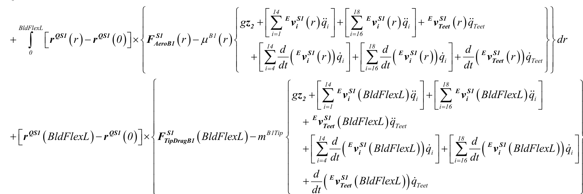
MBH1(0 )= AMe1roB1(r ) dr+ rQS1(r )−rQS1(0 )×FASe1roB1(r )−µB1(r ) gz2−µB1(r )EaS1(r )dr +rQS1(BldFlexL)−rQS1(0 )×{FTSip1DragB1(BldFlexL)−mB1Tipgz2+EaS1(BldFlexL)}

\begin{array}{r}{\stackrel{\mathrm{tora}}{\left\{F_{A e r o B l}^{S I}\left(r\right)-\mu^{B I}\left(r\right)\left\{\begin{array}{l}{g z_{2}+{^{E}}\nu_{_{I}}^{S I}\left(r\right)\vec{q}_{I}+\left[\sum_{i=l}^{H}E_{\nu_{i}}^{S I}\left(r\right)\vec{q}_{i}\right]+\left[\sum_{i=l}^{l,B}E_{\nu_{i}}^{S I}\left(r\right)\vec{q}_{i}\right]+\frac{E}{\nu_{_{I}}}\nu_{_{I}\infty}^{S I}}\\ {\qquad-\left[\displaystyle\sum_{i=l}^{H}\frac{d}{d t}\left({^{E}}\nu_{_{i}}^{S I}\left(r\right)\right)\vec{q}_{i}\right]+\left[\sum_{i=l\infty}^{[B}\frac{d}{d t}\left({^{E}}\nu_{_{i}}^{S I}\left(r\right)\right)\vec{q}_{i}\right]+\frac{d}{d t}\left({^{E}}\nu_{_{I e r}}^{S I}\left({^{\phantom{-}}\vec{q}_{i}\right)\vec{q}_{i}\right]+}\end{array}\right.}}\\ {\stackrel{\mathrm{tor~}}{\left.+\left.F_{r\mu\rho\rho\mu\lambda}^{S I}\left(B I d F l e x L\right)-m^{B I\pi}\right]\left\{\mathcal{G}z_{2}+\left[\sum_{i=l}^{\mathcal{M}}E_{\nu_{i}}^{S I}\left(B I d F l e x L\right)\vec{q}_{i}\right]+\left[\sum_{i=l\infty}^{[B}E_{\nu_{i}}^{S I}\left(B I d F l e x L\right)\vec{q}_{i}\right]\right]+\left[\sum_{i=l\infty}^{B}E_{\nu_{i}}^{S I}\left(B I d F l e x L\right)\vec{q}_{i}\right]\right\}}_{\alpha}}\end{array}\right.

M_{B I}^{H}\left(0\right)=\int_{0}^{B l d F l e x L}M_{A e r o B I}^{M I}\left(r\right)d r

FBS11t(0 ) \begin{array}{c}{{^{L}\mu^{B I}\left(r\right)^{E}\nu_{r}^{S I}\left(r\right)d r-m^{B I T p}~\nu_{r}^{S I}\left(B I d F l e x L\right)}}\\ {{\mathrm{}}}\\ {{\displaystyle\left\{F_{A e e n I}^{S I}\left(r\right)-\mu^{B I}\left(r\right)\left\{g z_{2}+\left[\sum_{i=4}^{M}\frac{d}{d t}\left(^{\varepsilon}\nu_{i}^{S I}\left(r\right)\right)\dot{q}_{i}\right]+\left[\sum_{i=l6}^{l8}\frac{d}{d t}\left(^{\varepsilon}\nu_{i}^{S I}\left(r\right)\right)\dot{q}_{i}\right]+\frac{d}{d t}\left(^{\varepsilon}\nu_{{r e e}}^{S I}\left(r\right)\right)\right\}\left(^{\varepsilon}\mu^{B}\right)\right\}~}}\\ {{\displaystyle B I T p\left\{g z_{2}+\left[\sum_{i=d}^{M}\frac{d}{d t}\left(^{\varepsilon}\nu_{i}^{S I}\left(B I d F l e x L\right)\right)\dot{q}_{i}\right]+\left[\sum_{i=l6}^{l8}\frac{d}{d t}\left(^{\varepsilon}\nu_{{b}}^{S I}\left(B I d F l e x L\right)\right)\dot{q}_{i}\right]+\frac{d}{d t}\left(^{\varepsilon}\nu_{{r e e}}^{S I}\left(1-{\cal E}\right)\right)\right\}~}}\\ {{\displaystyle\left\{s!I\right.}}\end{array} r ))qTeet dr −mB1Tip BldFlexL))qTee + FS FTSip1DragB1(BldFlexL)

MBH1r(0 )= − ∫ rQS1(r )−rQS1(0 )×µB1(r )EvrS1(r )dr−mB1TiprQS1(BldFlexL)−rQS1(0 )×EvrS1(BldFlexL) (r=1,2,,14;16,17,18;Teet)
MBH1t(0 )= ∫ rQS1(r )−rQS1(0 )×FASe1roB1(r )−µB1(r )gz2+1∑4 ddt(EviS1(r ))qi+ \sum_{i=l6}^{l\delta}\frac{d}{d t}\Big(^{E}\nu_{i}^{s t}\left(r\right)\Big)\dot{q}_{i} +ddt(EvTSe1et(r ))qTeetdr gz2+1∑4 ddt(EviS1(BldFlexL))qi+1∑8 ddt(EviS1(BldFlexL))qi +rQS1(BldFlexL)−rQS1(0 )×FTSip1DragB1(BldFlexL)−mB1Tip + d (EvTSe1et(BldFlexL))qTeet BldFlexL MAMe1roB1(r ) dr

The output loads are as follows:

RootFxc1=FBS11(0 )⋅i1B1/ 1,000 R o o t F y c l=F_{B I}^{S I}\left(0\right)\cdot\dot{\pmb{t}}_{2}^{B I}\,/\,l,000 R o o t F x b I=F_{B I}^{S I}\left(0\right)\cdot\pmb{j}_{I}^{B I}\,/\,I,000 R o o t F y b I=F_{B I}^{S I}\left(0\right)\cdot\pmb{j}_{2}^{B I}\,/\,I,0O0

Blade 1 OoP shear force at the blade root (directed along the xc1-axis), (kN) Blade 1\;\mathrm{IP} shear force at the blade root (directed along the yc1-axis), (kN) Blade 1 flapwise shear force at the blade root (directed along the xb1-axis), (kN) Blade 1 edgewise shear force at the blade root (directed along the yb1-axis), (kN)

R o o t F z c l=R o o t F z b I=F_{B I}^{S I}\left(O\right)\cdot\dot{\imath}_{3}^{B I}\mathrm{~/~}l,O O O=F_{B I}^{S I}\left(O\right)\cdot\dot{\jmath}_{3}^{B I}\mathrm{~/~}l,O O O

Blade 1 axial force at the blade root (directed along the zc1-/zb1-axis), (kN)

R o o t M x c l=R o o t M I P l=M_{B I}^{H}\left(\boldsymbol{\theta}\right)\cdot\dot{\boldsymbol{\imath}}_{I}^{B I}\mathrm{~/~}l,000

Blade 1 IP moment (i.e., the moment caused by IP forces) at the blade root (about the xc1-axis),

R o o t M y c I=R o o t M O o P I=M_{B I}^{H}\left(0\right)\cdot\dot{\pmb{i}}_{2}^{B I}\mathrm{~/~}I,000

Blade 1 OoP moment (i.e., the moment caused by OoP forces) at the blade root (about the yc1-

R o o t M x b I=R o o t M E d g I=M_{B I}^{H}\left(\boldsymbol{\theta}\right)\cdot\dot{\boldsymbol{j}}_{I}^{B I}\mathrm{\Delta}/\mathit{I},000

Blade 1 edgewise moment (i.e., the moment caused by edgewise forces) at the blade root (about

R o o t M y b I=R o o t M F l p I=M_{B I}^{H}\left(\boldsymbol{\theta}\right)\cdot\dot{\boldsymbol{J}}_{2}^{B I}\mathrm{\textit{/}}I,000

Blade 1 flapwise moment (i.e., the moment caused by flapwise forces)at the blade root (about the

R o o t M z c I=R o o t M z b I=M_{B I}^{H}\left({\boldsymbol{\partial}}\right)\cdot{\dot{\boldsymbol{i}}}_{3}^{B I}\left/I,000=M_{B I}^{H}\left({\boldsymbol{\partial}}\right)\cdot{\dot{\boldsymbol{j}}}_{3}^{B I}\left/I,000\right. (\mathrm{kN}\!\cdot\!\mathrm{m})

Blade 1 pitching moment at the blade root (about the zc1-/zb1-axis),

Blade 1 Local Moment Outputs:

There are 3 output loads at any of the selected span stations i \mathbf{\zeta}(r=\,R^{s p a n\;i}\,\rightleftharpoons\,R^{s p a n\;i}\,\rightleftharpoons\,R^{s p a n\;i}\,, ) of blade 1 (i{=}1,\!2,\!...,\!5) . These are the 3 components of the bending moment M_{B I}^{M I}\left(R^{S p a n\;i}\right) expressed in the local blade coordinate system (principal structural axes). Examining the results for the blade 1 root loads, it follows that:

The output loads are as follows:

S p n i M L x b I=M_{B I}^{M I}\left(R^{S p a n\;i}\right)\cdot n_{I}^{B I}\left(R^{S p a n\;i}\right)/\,I,000 S p n i M L y b I=M_{B I}^{M I}\left(R^{S p a n\;i}\right)\cdot n_{2}^{B I}\left(R^{S p a n\;i}\right)/\,I,000 \mathit{S p n i M L z b l}=M_{\mathit{B I}}^{\mathit{M I}}\left(R^{\mathit{S p a n\;i}}\right)\cdot n_{3}^{\mathit{B I}}\left(R^{\mathit{S p a n\;i}}\right)/\mathit{I,O00}

Blade 1 local edgewise moment at span station i (about the local xb1-structural axis), (\mathrm{kN}\!\cdot\!\mathrm{m}) Blade 1 local flapwise moment at span station i (about the local yb1-structural axis), (\mathrm{kN}\!\cdot\!\mathrm{m}) Blade 1 pitching moment at span station i (about the zc1-/zb1-/local zb1-axis), (\mathrm{kN\cdotm})

Blade 2 Root Loads: The equations for F_{B2}^{S2}\left(0\right),\;M_{B2}^{H}\left(0\right),\;F_{B2_{r}}^{S2}\left(0\right),\;F_{B2_{t}}^{S2}\left(0\right),\;M_{B2_{r}}^{H}\left(0\right),\;M_{B2_{t}}^{H}\left(0\right) , and all 10 output loads are similar to blade 1.

Hub and Rotor Loads:

There are 14 output loads at the hub end of the low-speed shaft. 5 of them are the 3 components of the thrust and shear force F_{R o t o r}^{P} (2 components are expressed in a nonrotating frame, 2 components are expressed in a rotating frame, and 1 component is independent of rotation). 5 other loads are the 3 components of the shaft bending moments, M_{R o t o r}^{L@P} (again, 2 components are expressed in a nonrotating frame, 2 components are expressed in a rotating frame, and 1 component is independent of rotation). The 11^{\mathrm{th}} and 12^{\mathrm{th}} loads are the rotor power and rotor power coefficient, respectively. The 13^{\mathrm{th}} and 14^{\mathrm{th}} loads are the rotor thrust and rotor torque coefficients, respectively. For a 2-blader, all these loads are given relative to the teeter pin (point P) as indicated. For the 3-blader, all of these loads are given relative to the apex of rotation (point Q, which is coincident with point P). The new generalized active force for the equations of motion resulting from these new loads is:

F_{r}\big|_{R o t o r}={^{E}\pmb{\nu}}_{r}^{P}\cdot F_{R o t o r}^{P}+{^{E}\pmb{\omega}}_{r}^{L}\cdot M_{R o t o r}^{L@P}\quad\left(r=l,2,...,22\right)

This generalized active force must produce the same effects as the generalized active and inertia forces associated with blade 1, blade 2, the hub, and the teeter springs and dampers. Thus,

\begin{array}{r l}&{F_{r}\big|_{R o t o r}=F_{r}^{*}\big|_{B I}+F_{r}\big|_{A e r o B I}+F_{r}\big|_{G r a v B I}+F_{r}\big|_{E l a s t i c B I}+F_{r}\big|_{D a m p B I}}\\ &{~+F_{r}^{*}\big|_{B_{2}}+F_{r}\big|_{A e r o B2}+F_{r}\big|_{G r a v B2}+F_{r}\big|_{E l a s t i c B2}+F_{r}\big|_{D a m p B2}}&{\big(r=I,2,\dots,22\big)}\\ &{~+F_{r}^{*}\big|_{H}+F_{r}\big|_{G r a v H}+F_{r}\big|_{S p r i n g T e e t}+F_{r}\big|_{D a m p T e e t}}\end{array}

Since ^E_{\nu_{r}^{P}} and \varepsilon_{\pmb{\omega}_{r}^{L}} are equal to zero unless r=1,2,...,14 , the generalized active forces associated with blade and teeter elasticity and damping do not contribute to the hub and rotor loads (since also, F_{r}|_{E l a s t i c B I}\,,\;F_{r}|_{D a m p B I}\,,\;F_{r}|_{E l a s t i c B2}\,,\;F_{r}|_{D a m p B2}\,,\;F_{r}|_{S p r i n g T e e}\,. , and F_{r}|_{D a m p T e e t} are equal to zero if r= 1,2,…,14). So,

F_{r}\Big|_{R o t o r}=F_{r}^{*}\Big|_{B I}+F_{r}\Big|_{A e r o B I}+F_{r}\Big|_{G r o w B I}+F_{r}^{*}\Big|_{B2}+F_{r}\Big|_{A e r o B2}+F_{r}\Big|_{G r o w B2}+F_{r}^{*}\Big|_{H}+F_{r}\Big|_{G r o w B}\quad(r=0,1)

When using the results for the blade 1 and blade 2 root loads, this equation can be simplified as follows:

F_{r}\big|_{R o t o r}=F_{r}\big|_{B I}+F_{r}\big|_{B2}+F_{r}^{*}\big|_{H}+F_{r}\big|_{G r a v H}\quad\big(r=I,2,...,I\mathcal{I}\big)

Thus,

\begin{array}{r l}&{\mathbf{\Xi}_{B I}^{S I}\left(\theta\right)+}\\ &{\mathbf{\Xi}_{B I}^{E}\left(\theta\right)+}\\ &{\varepsilon_{\nu}^{C}\cdot\left({\vphantom{\int_{0}^{\tau}}}\varepsilon_{a}^{C}+g\varepsilon_{2}\right)-}\end{array}\!\!\!\!\!\!\!\!\!\!\!\!\!\!\!\!\!\!\!\left({\cal M}_{B I}^{H}\left(\theta\right)+\left[r^{\underline{{{\theta}}}S I}\left(\theta\right)-r^{\underline{{{\theta}}}C}+\right]\times{\cal F}_{B I}^{S I}\left(\theta\right)\right\}+{\vphantom{\int_{0}^{\tau}}}{\varepsilon_{\nu}^{C}}\cdot{\cal F}_{B2}^{S2}\left(\theta\right)+}\\ &{\varepsilon_{\nu}^{C}\cdot\left({\vphantom{\int_{0}^{\tau}}}\varepsilon_{a}^{C}+g\varepsilon_{2}\right)-}\varepsilon_{\omega_{r}^{H}}\cdot\left(\overline{{{\cal I}}}^{H}\cdot{\vphantom{\int_{0}^{\tau}}}\alpha_{\nu}^{H}+{\vphantom{\int_{0}^{\tau}}}\omega^{H}\times\overline{{{\cal I}}}^{H}\cdot{\vphantom{\int_{0}^{\tau}}}\omega^{H}\right)}\end{array}

or when grouping like terms:

\begin{array}{l}{{\overline{{{F}}}_{B I}^{S I}\left(\boldsymbol{\theta}\right)+F_{B2}^{S2}\left(\boldsymbol{\theta}\right)-m^{H}\left(\frac{\varepsilon}{\varepsilon}{a}^{c}+g\varepsilon_{2}\right)\right]}}\\ {{{\mathbf{\nabla}^{\prime}}\cdot\left\{M_{B I}^{H}\left(\boldsymbol{\theta}\right)+M_{B2}^{H}\left(\boldsymbol{\theta}\right)+\left[r^{Q S I}\left(\boldsymbol{\theta}\right)-r^{Q C}\right]\times F_{B I}^{S I}\left(\boldsymbol{\theta}\right)+\left[r^{Q S2}\left(\boldsymbol{\theta}\right)-r^{Q C}\right]\times F_{B2}^{S2}\left(\boldsymbol{\theta}\right)-\overline{{{\overline{{{I}}}}}}^{H}\mathbf{\nabla}^{E}\right\}}}\end{array}

Recognizing that EvrC =EvrP EωH×(rPQ+rQC) , this generalized force can be expanded to:

\begin{array}{r l}&{^{E}\nu_{r}^{P}+^{E}\omega_{r}^{H}\times\left(r^{P Q}+r^{Q C}\right)\Biggr]\cdot\left[F_{B I}^{S I}\left(\theta\right)+F_{B2}^{S2}\left(\theta\right)-m^{H}\left(^{E}a^{C}+g z_{2}\right)\Biggr]}\\ &{+^{E}\omega_{r}^{H}\cdot\Bigl\{M_{B I}^{H}\left(\theta\right)+M_{B2}^{H}\left(\theta\right)+\left[r^{Q S I}\left(\theta\right)-r^{Q C}\right]\times F_{B I}^{S I}\left(\theta\right)+\Bigl[r^{Q S2}\left(\theta\right)-r^{Q C}\Bigr]\times F_{B2}^{S2}\left(\theta\right)-^{\frac{1}{2}}}\end{array}

Now applying the cyclic permutation law of the scalar triple product:

\begin{array}{r l}&{{\nu_{r}^{P}}\cdot\left[F_{B I}^{S I}\left(\theta\right)+F_{B2}^{S2}\left(\theta\right)-m^{H}\left({}^{E}a^{C}+{g}{z_{2}}\right)\right]+{}^{E}\omega_{r}^{H}\cdot\left\{\left(r^{P Q}+r^{Q C}\right)\times\left[F_{B I}^{S I}\left(\theta\right)+F_{B2}^{S2}\left(\theta\right)-F_{B I}^{S I}\left(\theta\right)\right]\right\}}\\ &{+{}^{E}\omega_{r}^{H}\cdot\left\{M_{B I}^{H}\left(\theta\right)+M_{B2}^{H}\left(\theta\right)+\left[r^{Q S I}\left(\theta\right)-r^{Q C}\right]\times F_{B I}^{S I}\left(\theta\right)+\left[r^{Q S2}\left(\theta\right)-r^{Q C}\right]\times F_{B2}^{S2}\left(\theta\right)-\frac{1}{L}\omega_{r}^{H}\left(\theta\right)\right\}}\end{array}

which simplifies to:

\left.\begin{array}{l}{{\cdot\left[F_{B I}^{S I}\left(\theta\right)+F_{B^{2}}^{S2}\left(\theta\right)-m^{H}\left(^{E}{\boldsymbol{a}}^{C}+g z_{2}\right)\right]}}\\ {{\omega_{r}^{H}\cdot\left\{\begin{array}{l}{{M_{B I}^{H}\left(\theta\right)+M_{B^{2}}^{H}\left(\theta\right)+\left[r^{P Q}+r^{\vartheta S I}\left(\theta\right)\right]\times F_{B I}^{S I}\left(\theta\right)+\left[r^{P Q}+r^{\vartheta S2}\left(\theta\right)\right]\times F_{B^{2}}^{S2}\left(\theta\right)}}\\ {{-m^{H}\left(r^{P Q}+r^{Q C}\right)\times\left(^{E}{\boldsymbol{a}}^{C}+g z_{2}\right)-\overline{{{\overline{{{I}}}}}}\cdot{\boldsymbol{\varepsilon}}_{\alpha}^{E}{\boldsymbol{a}}^{H}-{^{E}}\omega^{H}\times\overline{{{\overline{{{I}}}}}}^{H}\cdot{^{E}}\omega^{H}}}\end{array}\right\}}}\end{array}\left(r\right)}

However, ^E_{\omega_{r}^{H}} equals ^E\pmb{\omega}_{r}^{L} when r is not equal to Teet. Thus the generalized active force associated with the rotor can be expressed as follows:

\begin{array}{r l}&{=^{E}\nu_{r}^{P}\cdot\left[F_{B I}^{S I}\left(\theta\right)+F_{B2}^{S2}\left(\theta\right)-m^{H}\left(^{E}a^{C}+g z_{2}\right)\right]}\\ &{\phantom{=}+^{E}\omega_{r}^{L}\cdot\left\{\begin{array}{l l}{M_{B I}^{H}\left(\theta\right)+M_{B2}^{H}\left(\theta\right)+\left[r^{P Q}+r^{Q S I}\left(\theta\right)\right]\times F_{B I}^{S I}\left(\theta\right)+\left[r^{P Q}+r^{Q S2}\left(\theta\right)\right]\times F_{B2}^{S2}\left(\theta\right)}\\ {\phantom{=}-m^{H}\left(r^{P Q}+r^{Q C}\right)\times\left(^{E}a^{C}+g z_{2}\right)-\overline{{\bar{I}}}^{H}\cdot^{E}\alpha^{H}-^{E}\omega^{H}\times\overline{{\bar{I}}}^{H}\cdot^{E}\omega^{H}}\end{array}\right.}\end{array}

Thus it is seen that,

F_{R o t o r}^{P}=F_{B I}^{S I}\left(0\right)+F_{B2}^{S2}\left(0\right)-m^{H}\left({}^{E}a^{C}+g z_{2}\right)

MRLo@toPr=MBH1(0 )+MBH2(0 )+rPQ+rQS1(0 )×FBS11(0 )+rPQ+rQS2(0 )×FBS22(0 )−mH(rPQ+rQC) ( a +gz2)−I a −EωH×IH⋅Eω Thus,

\mathbf{\Psi}_{R o t o r}^{P}=F_{B I}^{S I}\left(\boldsymbol{\theta}\right)+F_{B2}^{S2}\left(\boldsymbol{\theta}\right)-m^{H}\left\{\left(\sum_{i=I}^{H}E_{\nu_{i}^{C}}\hat{q}_{i}\right)+\;E_{\nu_{T e t}^{C}}\hat{q}_{T e e t}+\left[\sum_{i=I}^{H}\frac{d}{d t}\Big(\boldsymbol{\varepsilon}\nu_{i}^{C}\Big)\hat{q}_{i}\right]+\frac{d}{d t}\Big(\boldsymbol{\varepsilon}\nu_{T e t}^{C}\hat{q}_{i}\Big)\right\},

\begin{array}{c}{{\displaystyle\Gamma_{R o t o r}^{A\bar{\alpha}P}=M_{B I}^{H}\left(\theta\right)+M_{B2}^{H}\left(\theta\right)+\left[r^{P Q}+r^{Q S I}\left(\theta\right)\right]\times F_{B I}^{S I}\left(\theta\right)+\left[r^{P Q}+r^{Q S2}\left(\theta\right)\right]\times F_{B2}^{S2}\left(\theta\right)}}\\ {{\displaystyle-m^{H}\left(r^{P Q}+r^{Q C}\right)\times\left\{\left(\sum_{i=I}^{I\!\!\!/}^{k}{\varepsilon_{\nu}}_{i}^{C}\ddot{q}_{i}\right)\!\!+{}^{E}{\nu}_{{\nu}\!\!\!/e c t}^{C}\ddot{q}_{{\mathrm{ref}}}\!\!+\!\left[\sum_{i=I}^{I\!\!\!/}\frac{d}{d t}\!\left({}^{E}\nu_{{\nu}\!\!\!/}^{C}\right)\dot{q}_{i}\right]\!\!+\!\frac{d}{d t}\!\left({}^{E}\nu_{{\nu}\!\!\!/e c t}^{C}\right)\dot{q}_{i}\right.}}\\ {{\displaystyle-\overline{{{\cal F}}}^{H}\cdot\left\{\left(\sum_{i=I}^{I\!\!\!/}{}^{E}{\varepsilon_{\nu}}_{i}^{H}\ddot{q}_{i}\right)\!\!+{}^{E}{\omega}_{I e r t}^{H}\ddot{q}_{{\mathrm{ref}}}\!\left.+\!\left[\sum_{i=I}^{I\!\!\!/}\frac{d}{d t}\!\left({}^{E}{\omega}_{i}^{H}\right)\dot{q}_{i}\right]\!\!+\!\frac{d}{d t}\!\left({}^{E}{\omega}_{{\nu}\!\!\!/e c t}^{H}\right)\dot{q}_{{\mathrm{ref}}}\right\}-{}^{E}{\omega}_{I}}}\end{array}

Or,

\begin{array}{l}{{\displaystyle F_{R o t o r_{r}}^{P}=F_{B I_{r}}^{S I}\left(\boldsymbol{\theta}\right)+F_{B2_{r}}^{S2}\left(\boldsymbol{\theta}\right)-m^{H}^{\textit{E}}\pmb{\nu}_{r}^{c}\quad\left(r=I,2,\ldots,I\mathcal{I};I6,I7,\ldots,22\right)}}\\ {{\displaystyle F_{R o t o r_{t}}^{P}=F_{B I_{t}}^{S I}\left(\boldsymbol{\theta}\right)+F_{B2_{t}}^{S2}\left(\boldsymbol{\theta}\right)-m^{H}\left\{\left[\sum_{i=d}^{M}\frac{d}{d t}\!\left(^{\varepsilon}\nu_{i}^{c}\right)\boldsymbol{\dot{q}}_{i}\right]\!+\!\frac{d}{d t}\!\left(^{\varepsilon}\nu_{{I}\!e e t}^{c}\right)\boldsymbol{\dot{q}}_{{T e e t}}+g\boldsymbol{z}_{2}\right\}}}\end{array}

\begin{array}{l}{{{\cal M}_{R o t o r_{r}}^{L@P}={\cal M}_{B_{I_{r}}}^{H}\left(0\right)+{\cal M}_{B_{2r}}^{H}\left(\theta\right)\mathrm{+}\left[r^{P Q}+r^{Q S I}\left(0\right)\right]\times F_{B{I_{r}}}^{S I}\left(\theta\right)\mathrm{+}\left[r^{P Q}+r^{Q S2}\left(\theta\right)\right]\times F_{B{I_{r}}}^{S2}\left(\theta\right)}}\\ {{{\cal M}_{R o t o r_{t}}^{L@P}={\cal M}_{B_{I_{r}}}^{H}\left(\theta\right)\mathrm{+}{\cal M}_{B_{2\mathrm{t}}}^{H}\left(\theta\right)\mathrm{+}\left[r^{P Q}+r^{Q S I}\left(\theta\right)\right]\times F_{B{I_{r}}}^{S I}\left(\theta\right)\mathrm{+}\left[r^{P Q}+r^{Q S2}\left(\theta\right)\right]\times F_{B{I_{r}}}^{S2}\left(\theta\right)}}\\ {{\mathrm{\quad~}}}\\ {{{\displaystyle~~-\,\overline{{\cal I}}^{H}\cdot\left\{\left[\sum_{i=7}^{M}\frac{d}{d t}\Big({}^{E}\omega_{i}^{H}\Big)\dot{q}_{i}\right]\!\!+\!\frac{d}{d t}\Big({}^{E}\omega_{T e t}^{H}\Big)\dot{q}_{T e t}\Big\}\!\!-{}^{E}\omega^{H}\times\overline{{\cal I}}^{H}\cdot{}^{E}\omega^{H}}}}\end{array} −mH(rPQ+rQC) EωH (r=1,2,,14;16,17,, −mH(rPQ+rQC)×1∑4 ddt(EviC)qi+ddt(EvTCeet)qTeet+gz2

The output loads are as follows,

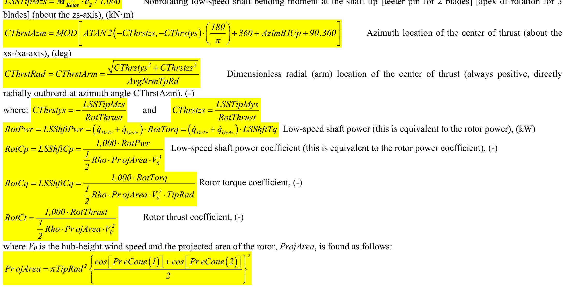
R o t T h r u s t=L S S h f t F x s=L S S h f t F x a=F_{R o t o r}^{P}\cdot e_{I}\;/\;I,000=F_{R o t o r}^{P}\cdot c_{I}\;/\;I,000 is constant along the shaft and is equivalent to the rotor thrust force), (\mathrm{kN})

Low-speed shaft thrust force (directed along the xs-/xa-axis) (this

L S S h f t F y a=F_{R o t o r}^{P}\cdot e_{2}\ ⁄I,O O O L S S h f t F z a=F_{R o t o r}^{P}\cdot e_{3}\,/\,l,000 L S S h f t F y s=-F_{R o t o r}^{P}\cdot c_{s}\,/\,l,000 L S S h f t F z s=F_{R o t o r}^{P}\cdot c_{2}\mathit{\Omega}/{I,O O O}

Rotating low-speed shaft shear force (directed along the ya-axis) (this is constant along the shaft), (kN) Rotating low-speed shaft shear force (directed along the za-axis) (this is constant along the shaft), (kN) Nonrotating low-speed shaft shear force (directed along the ys-axis) (this is constant along the shaft), (kN) Nonrotating low-speed shaft shear force (directed along the zs-axis) (this is constant along the shaft), (kN)

RotT \diamond r q=L S S h f t T q=L S S h f t M x s=L S S h f t M x a=M_{\cal R o t o r}^{L a P}\cdot e_{I}\;/\;I,\theta\theta0=M_{\cal R o t o r}^{L a P}\cdot e_{I}\;/\;I,\theta\theta0=0,\forall01\theta\in\cal R^{3}:\cal R^{3}. Low-speed shaft torque (about the xs-/xa-axis) (this is constant along the shaft and is equivalent to the rotor torque), (\mathrm{kN\cdotm})

L S S T i p M y a=M_{R o t o r}^{L@P}\cdot e_{2}\;/\;l,O O O (about the ya-axis), (\mathrm{kN\cdotm}) L S S T i p M z a=M_{R o t o r}^{L@P}\cdot e_{3}\,/\,l,000 (about the za-axis), (\mathrm{kN}\!\cdot\!\mathrm{m})

Rotating low-speed shaft bending moment at the shaft tip [teeter pin for 2 blades] [apex of rotation for 3 blades]

Rotating low-speed shaft bending moment at the shaft tip [teeter pin for 2 blades] [apex of rotation for 3 blades]

L S S T i p M y s=-M_{R o t o r}^{L@P}\cdot c_{s}\,/\,I,O O O blades] (about the ys-axis), (\mathrm{kN\cdotm})

Nonrotating low-speed shaft bending moment at the shaft tip [teeter pin for 2 blades] [apex of rotation for 3

L S S T i p M z s=M_{R o t o r}^{L@P}\cdot c_{2}\;/\;l,000

The rotor torque is equal to low-speed shaft torque as seen above. It is noted that this torque can be computed differently using the drivetrain flexibility and damping, though the load summation method and this other constraint method are equivalent. This can be demonstrated as follows. First of all, the equation above is equivalent to saying:

L S S h f t T q={}^{E}\omega_{D r T r}^{L}\cdot M_{R o t o r}^{L@P}\slash{I},000

However, since ^E_{\nu_{D r T r}^{P}} is equal to zero, it is also equivalent to say:

\begin{array}{l}{{^{E}\nu_{_{D r T}}^{P}\cdot F_{_{R o t o r}}^{P}+^{\varepsilon}\omega_{D r T}^{L}\cdot M_{R o t o r}^{L\ @P}}}\\ {\mathrm{~}}\\ {{^{\sum_{\substack{J r\sim\Gamma}}}\left|_{R o t o r}/\mathit{I},000\right.\mathrm{~or}\qquad L S S h/t{\Gamma q}=\left(F_{_{D r T}}^{\ast}\Big|_{B I}+F_{D r T}\Big|_{A e r o B I}+F_{D r T}\Big|_{G r a v B I}+F_{D r T}^{\ast}\Big|_{B J}+F_{D r r}\Big|_{B I}\right)}}\end{array}

From the equations of motion, it is easily seen that this is equivalent to saying:

\begin{array}{r}{L S S h f t T q=\left(-F_{D r T r}\right|_{E l a s t i c D r i v e}-F_{D r T r}\Big|_{D a m p D r i v e}\right)/{\mathit{I}},000}\end{array}

and thus,

\begin{array}{r l}{L S S h f t T q=\left(D T T o r S p r\cdot q_{D r T}+D T T o r D m p\cdot\dot{q}_{D r T r}\right)/\,I,000}&{\left(=\,M_{R o t o r}^{L a P}\cdot c_{I}\,/\,I,000\right)}\end{array} and is equivalent to the rotor torque)

Thus, both the load summation method and the constraint method are equivalent. However, if the drivetrain DOF is disabled, then q_{D r T r} will equal zero and \dot{q}_{D r T r} will equal zero, which implies that, at least, DTTorSpr is equal to infinity (since the product of DTTorSpr and q_{D r T r} is, in general, nonzero). Thus, to avoid using 2 different methods to calculate LSShftTq , it is best just to use M_{R o t o r}^{L@P}\cdot c_{I}\,/\,I,O O O , which will always work, regardless of the number of DOFs disabled.

Like the LSShftTq , it is noted that LSSTipMya can also be computed differently using the teeter springs and dampers, though the load summation method and this other constraint method are equivalent. This also can be demonstrated as follows. First of all, the equation above is equivalent to saying:

L S S T i p M y a=\mathit{\Pi}^{E}\omega_{T e e t}^{H}\cdot M_{R o t o r}^{L@P}\mathit{\Pi}/\mathit{I},000

Or,

M\!y a={}^{E}\!\omega_{T e e t}^{H}\cdot\left\{\!M_{B I}^{H}\left(\theta\right)\!+\!M_{B2}^{H}\left(\theta\right)\!+\!\left[{r}^{P Q}+{r}^{Q S I}\left(\theta\right)\right]\!\times\!F_{B I}^{S I}\left(\theta\right)\!+\!\left[{r}^{P Q}+{r}^{Q S2}\left(\theta\right)\right]\!\times\!F_{B2}^{S I}\left(\theta\right)\!+\!\left[{r}^{P Q}\right]\!+\!{r}^{Q S2}\left(\theta\right)\!\right]\!\times\!F_{B2}^{S I}\left(\theta\right)\!+\!{r}^{P Q}\left(\theta\right)^{2},

Now applying the cyclic permutation law of the scalar triple product:

\begin{array}{l}{{^{E}\omega_{T e t}^{H}\times\left[r^{P Q}+r^{Q S I}\left(0\right)\right]\cdot F_{B I}^{S I}\left(0\right)+^{E}\omega_{3}^{H}\times\left[r^{P Q}+r^{Q S2}\left(0\right)\right]\cdot F_{B2}^{S2}\left(0\right)-m^{H}\,^{E}\omega_{T e t}^{H}\times\left(r^{P Q}+r^{Q S2}\left(0\right)\right)}}\\ {{\mathrm{}\,\,\,\,\,+\,\,^{E}\omega_{T e t}^{H}\cdot\left[M_{B I}^{H}\left(0\right)+M_{B2}^{H}\left(0\right)-\overline{{{\overline{{{I}}}}}}\,^{H}\cdot^{E}\alpha^{H}-^{E}\omega^{H}\times\overline{{{\overline{{{I}}}}}}\,^{H}\cdot^{E}\omega^{H}\right]}}\end{array}

Recognizing also that E_{\psi_{I e e t}}^{\phantom{\dagger}}\left(\theta\right)={}^{E}\omega_{I_{e e t}}^{H}\times\left[r^{P Q}+r^{Q S I}\left(\theta\right)\right]\quad,\qquad\quad{}^{E}\nu_{I_{e e t}}^{S2}\left(\theta\right)={}^{E}\omega_{I_{e e t}}^{H}\times\left[r^{P Q}+r^{Q S2}\left(\theta\right)\right],\quad\forall\theta\in\mathbb{R}^{3}. nd {^E}{\nu}_{T e e t}^{C}={^E}\omega_{T e e t}^{H}\times\left(r^{P Q}+r^{Q C}\right) , this can be simplified as follows:

\begin{array}{r l}&{\frac{\nu I}{\nu e t}\left(\partial\right)\cdot F_{s t l}^{S I}\left(\partial\right)+^{E}\omega_{2r e t}^{H}\cdot M_{B I}^{H}\left(\partial\right)+^{E}\nu_{T e e t}^{S2}\left(\partial\right)\cdot F_{s t2}^{S2}\left(\partial\right)+^{E}\omega_{T e t}^{H}\cdot M_{B2}^{H}\left(\partial\right)-m^{H}^{E}\nu_{T e t}^{C}\cdot\left(^{L}\nu_{T e e t}^{C}\cdot M_{B2}^{H}\left(\partial\right)\right)}\\ &{-^{E}\omega_{T e t}^{H}\cdot\left(\overline{{\overline{{I}}}}^{H}\cdot^{E}\alpha^{H}+^{E}\omega^{H}\times\overline{{\overline{{I}}}}^{H}\cdot^{E}\omega^{H}\right)}\\ &{\qquad\qquad\times\left(\left|_{B I}+F_{T e e t}\right|_{B2}+F_{T e e t}^{*}\right|_{H}+F_{T e e t}\right|_{G r a b l}\right)/I,000}\\ &{\left.\left|_{t}\right|_{H}+F_{T e e t}^{*}\right|_{B I}+F_{T e e t}^{*}\right|_{B2}+F_{T e e t}^{*}\right|_{A e r o B l}+F_{T e e t}\Big|_{G r a b l}+F_{T e e t}\Big|_{G r a b l}+F_{T e e t}\Big|_{G r a b l}+F_{T e e t}\Big|_{G r a b l}}\end{array}

From the equations of motion, it is easily seen that this is equivalent to saying:

\begin{array}{r}{L S S T i p M y a=\left(-F_{T e e t}\vert_{S p r i n g T e e t}-F_{T e e t}\vert_{D a m p T e e t}\right)/\,I,000}\end{array}

and thus,

r i p M y a=\left\{\begin{array}{l l}{I F\Big[\Big|q_{T e e l}\Big|>T e e t S S t P,T e e t S S P\cdot S I G N\big(q_{T e e l}\Big)\Big(\Big|q_{T e e l}\Big|-T e e t S S t P\Big),0\Big]}\\ {+I F\Big[\Big|q_{T e e l}\Big|>T e e t H S t P,T e e t H S S p\cdot S I G N\big(q_{T e e l}\Big)\Big(\Big|q_{T e e l}\Big|-T e e t H S t P\Big),0\Big]}\\ {+I F\Big[\dot{q}_{T e e l}\bigtriangleup(0,T e e t C D m p\cdot S I G N\big(\dot{q}_{T e e l}\big),0\Big]+I F\Big[\Big|q_{T e e l}\Big|>T e e t D m p,T e e t C D m p\cdot}\end{array}\right].}\end{array}\right.

Thus, both the load summation method and the constraint method are equivalent. Thus, to avoid using 2 different methods to calculate LSSTipMya if various DOFs are disabled, it is best just to use M_{R o t o r}^{L@P}\cdot e_{2}\,/\,I,O O O , which will always work.

Shaft Strain Gage Loads:

There are 4 output loads at point SG on the low-speed shaft [which is a point on the shaft a distance ShftGagL towards the nacelle from point P (or point Q for a 3-blader since point \mathrm{P} does not exist)]. These are 2 of the 3 components of the shaft bending moments, M_{R o t o r}^{L@S G} (2 components are expressed in a nonrotating frame, 2 components are expressed in a rotating frame, and third component which is directed in the c_{I} direction is not used because it is the same as the rotor torque). Since the low-speed shaft is assumed to be rigid and massless between points \mathrm{P} and SG, it is easily seen that:

M_{R o t o r}^{L@S G}=M_{R o t o r}^{L@P}-r^{P S G}\times F_{R o t o r}^{P}

since r^{P S G} equals -r^{S G P} .

Thus,

L S S G a g M y a=M_{R o t o r}^{L@F}\cdot e_{2}\,/\,I,O00=L S S T i p M y a+S h f t G a g L\cdot L S S h f t F z a (about the ya-axis), (\mathrm{kN\cdotm})
\ L S S G a g M z a=M_{\scriptscriptstyle R o t o r}^{L@F}\cdot e_{_3}\cdot/\,I,O00=L S S T i p M z a-S h f t G a g L\cdot L S S h f t F y a (about the za-axis), (\mathrm{kN}\!\cdot\!\mathrm{m})
L S S G a g M y s=-M_{R o t o r}^{L@F}\cdot c_{3}\ /\ I,O O O=L S S T i p M y s+S h f t G a g L\cdot L S S h f t F z s (about the ys-axis), (\mathrm{kN}\!\cdot\!\mathrm{m})
L S S G a g M z s=M_{\scriptscriptstyle R o t o r}^{L@F}\cdot c_{_2}/I,000=L S S T i p M z s-S h f t G a g L\cdot L S S h f t F y s

Rotating low-speed shaft bending moment at the shaft’s strain gages Rotating low-speed shaft bending moment at the shaft’s strain gages Nonrotating low-speed shaft bending moment at the shaft’s strain gages Nonrotating low-speed shaft bending moment at the shaft’s strain gages

Note that no shear or thrust forces need be output at point SG since these would be the same as the shear and thrust forces at point P. Note also that

{c_{I}}\cdot{M_{R o t o r}^{L\left(\varpi P\right)}}={c_{I}}\cdot{M_{R o t o r}^{L\left(\varpi S G\right)}}

and thus the low-speed shaft torque or rotor torque are constant along the shaft.

Generator and High-Speed Shaft Loads:

There are 9 output loads on the high-speed shaft. The first and second are the high-speed shaft torque, HSShftTq , and high-speed shaft torque coefficient, HSShftCq , whose convention is that it has a positive value when the LSShftTq is positive. The third and fourth are the high-speed shaft power, HSShftPwr , and high-speed shaft power coefficient, H S S h f t C p . The fifth and sixth are the generator electrical torque, GenTq , and generator electrical torque coefficient, GenCq . The seventh is the high-speed shaft braking torque, HSSBrTq . The eighth is the generator electrical power, GenPwr . The ninth is the electrical generator power coefficient, GenCp .

From a simple free-body diagram of a black-box gearbox,

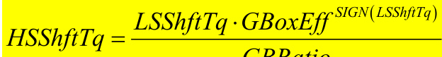
High-speed shaft torque (this is constant along the shaft and has the convention that it is positive

when the LSShftTq is positive), (kN·m)

This can alternatively be written in terms of the high-speed shaft motions and torques through use of the equation for the GeAz DOF as follows. From earlier work,

H S S h j t T q=\frac{\frac{E}{\omega_{D r T r}^{L}}\cdot M_{R o t o r}^{L@P}G B o x E\!f\!\!f^{S I G N\left(L S S h\!\!f t T q\right)}}{I,000\cdot G B R a t i o}

From the equations of motion for the GeAz DOF, it is seen that this is equivalent to saying:

H S S h f t T q=\frac{\left(-F_{G e d z}^{*}\Big|_{G}-F_{G e d z}\Big|_{G e n}-F_{G e d z}\Big|_{B r a k e}-F_{G e d z}\Big|_{G B F r i c}\right)G B o x E f f^{S I G N}(L S S h\beta t T q)}{I,O\theta O\cdot G B R a t i o}

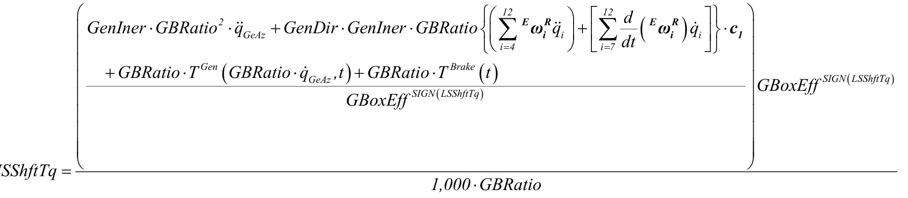
or,

HSShftTq =

or, HSShftTq=GenIner ⋅GBRatio⋅ qGeAz+GenDir ⋅GenInerEαR⋅c1+TGen(GBRatio ⋅qGeAz,t)+TBrake(t )/ 1,000

H S S h f t C q=\frac{I,O O O\cdot H S S h f t T q}{\frac{I}{2}R h o\cdot P r\,o j A r e a\cdot V_{o}^{2}\cdot T i p R a d}

H S S h j t P w r=H S S h j t T q\cdot G B R a t i o\cdot\dot{q}_{G e d z}

High-speed shaft power, (kW)

High-speed shaft power coefficient, (-)

H S S B r T q=T^{B r a k e}\left(t\right)/I,O O O

G e n T q=T^{G e n}\left(G B R a t i o\cdot\dot{q}_{G e d z},t\right)/\mathit{I},000 situation or power input), (\mathrm{kN\cdotm})

Electrical generator torque (positive reflects power extracted and negative represents a motoring-up

G e n C q\!=\!\frac{I,\!O00\cdot G e n T q}{\frac{I}{2}R h o\cdot P r\,o j\!A r e a\cdot V_{o}^{2}\cdot T i p R a d}

Electrical generator torque coefficient, (-)

Though the HSShftTq is calculated the same regardless of the generator model employed, GenPwr is not. Similar to how power is transmitted through the gearbox with a simple efficiency, for the simple generator or simple variable-speed generator control models, the electrical generator power is as follows:

G e n P w r=G B R a t i o\cdot\dot{q}_{G e,i z}\cdot G e n T q\cdot G e n E j f^{S I G N\left[T^{G e n}\left(G B R a t i o\cdot\dot{q}_{G e,i z},t\right)\right]}\;/\;I,0O0

Electrical generator power (positive reflects power extracted and negative

represents a motoring-up situation or power input), (kW)

And for the Thevenin-Equivalent induction generator model,

Electrical generator power (positive reflects power extracted and negative

represents a motoring-up situation or power input), (kW)

where, \begin{array}{r l}&{P w r_{_{M e c h a n i c a l}}=G B R a t i o\cdot\dot{q}_{_{G e d z}}\cdot T^{G e n}\left(G B R a t i o\cdot\dot{q}_{_{G e d z}},t\right)}\\ &{P w r_{_{S t a t o r L o s s}}=T E C_{-}N P h a\left|\overline{{I}}_{I}\right|^{2}T E C_{-}S\,R e s}\end{array}

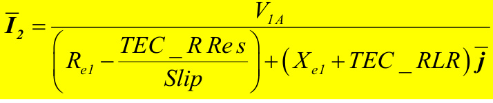
\overline{{{I}}}_{I}=\overline{{{I}}}_{2}+\frac{V_{I A}}{T E C\_M R\overline{{{j}}}}

(the sign of this is governed by T^{G e n} )

(always positive)

(always positive)

where the definition of V_{I a},R_{e I},X_{e I} , and Slip are given elsewhere and \overline{{\boldsymbol{j}}}=\sqrt{-\boldsymbol{l}} .

Otherwise, the electrical generator power, GenPwr, is a user-defined function of the high-speed shaft speed, GBRatio \dot{q}_{G e A z} , and time t .

Electrical generator power coefficient, (-)

Rotor-Furl Axis Loads:

There is 1 output load on the rotor-furl axis. This is the rotor-furl moment about the rotor-furl axis. Of course, we could also output all 6 components of the force F_{G e n,R o t}^{V}\ / moment M_{G e n,R o t}^{N\!(a V} acting on the rotor-furl axis at point V on the nacelle. Following the analysis for finding the blade root loads, the new generalized active force for the equations of motion resulting from these new loads is:

F_{r}|_{G e n,R o t}={}^{E}\nu_{r}^{V}\cdot F_{G e n,R o t}^{V}+{}^{E}\omega_{r}^{N}\cdot M_{G e n,R o t}^{N\overline{{\omega}}V}\quad\left(r=l,2,...,22\right)

This generalized active force must produce the same effects as the generalized active and inertia forces associated with blade 1, blade 2, the hub, the drivetrain, and the structure that furls with the rotor. Thus,

\begin{array}{r l}{\lefteqn{\mathrm{\partial_{r}=\}F_{r}^{*}\Big|_{B I}+F_{r}\Big|_{A e r o s h I}+F_{r}\Big|_{G r o w B I}+F_{r}\Big|_{E l a s t i c B I}+F_{r}\Big|_{D a m p B I}+F_{r}^{*}\Big|_{B2}+F_{r}\Big|_{A e r o B2}+F_{r}\Big|_{G r o w B2}+F_{r}\Big|_{E l a s t i c B}}\\ &{\quad+F_{r}^{*}\Big|_{H}+F_{r}\Big|_{G r o w H}+F_{r}\Big|_{S p r i n g T e e t}+F_{r}\Big|_{D a m p T e e t}+F_{r}^{*}\Big|_{G}+F_{r}\Big|_{G e n}+F_{r}\Big|_{B r a k e}+F_{r}\Big|_{G B F r i c}+F_{r}\Big|_{E l a s t i c}}\\ &{\quad+F_{r}^{*}\Big|_{R}+F_{r}\Big|_{G r o w B}+F_{r}\Big|_{S p r i n g R F}+F_{r}\Big|_{D a m p R F}}\end{array}

Since ^E\nu_{r}^{\nu} and ^E\pmb{\omega}_{r}^{N} are equal to zero unless r=1,2,...,11 , the generalized active forces associated with blade, drivetrain, rotor-furl, and teeter elasticity and damping, as well as the generator torque, HSS braking torque, and gearbox friction do not contribute to the rotor-furl loads (since also, Fr Ela _{s t i c B I},\;F_{r}\big|_{D a m p B I},\;F_{r}\big|_{E l a s t i c B},\;F_{r}\big|_{D a m p B2},\;F_{r}\big|_{S p r i n g T e e}\,,\;F_{r}\big|_{D a m p T e e t},\;F_{r}\big|_{S p r i n g R F}\,,\;F_{r}\big|_{D a m p R F}\,, ElasticDrive, Fr DampDrive, Fr Gen, Fr Brake, and F_{r}|_{G B F r i c} are equal to zero if r=1,2,...,11) . So,

FrGen,Ro ,={F_{r}^{*}}\Big|_{B I}+{F_{r}}\Big|_{A e r o B I}+{F_{r}}\Big|_{G r a v B I}+{F_{r}^{*}}\Big|_{B2}+{F_{r}}\Big|_{A e r o B2}+{F_{r}}\Big|_{G r a v B2}+{F_{r}^{*}}\Big|_{H}+{F_{r}}\Big|_{G r a v H}+{F_{r}^{*}}\Big|_{R}+{F_{r}}\Big|_{G r a v B} ravR+Fr*G (r=1,2,,11)

When using the results for hub and rotor loads, this equation can be simplified as follows:

F_{r}\big|_{G e n,R o t}=F_{r}\big|_{R o t o r}+F_{r}^{*}\big|_{R}+F_{r}\big|_{G r a v R}+F_{r}^{*}\big|_{G}\quad\big(r=I,2,...,I I\big)

Thus,

Fr Gen,Ro \v_{\tau}={}^{E}\nu_{r}^{P}\cdot F_{R o t o r}^{P}+{}^{E}\omega_{r}^{L}\cdot M_{R o t o r}^{L@P}-m^{R}{}^{E}\nu_{r}^{D}\cdot\left({}^{E}a^{D}+g z_{2}\right)-{}^{E}\omega_{r}^{R}\cdot\left({\overline{{{\overline{{I}}}}}}^{R}\cdot{}^{E}a^{R}+{}^{E}\omega^{R}\times{\overline{{{\overline{{I}}}}}}^{R}\cdot{}^{E}a^{R}\right) ωR)−EωrG⋅(IG⋅EαG+EωG×IG⋅EωG) (r=1,2,,11) However, {}^{E}{\pmb\omega}_{r}^{L}\,,\ {}^{E}{\pmb\omega}_{r}^{G}\,,\ {}^{E}{\pmb\omega}_{r}^{R} , and ^E\pmb{\omega}_{r}^{N} are all equal when r is constrained to be between 1 and 11. Thus, when grouping like terms:

{\bf\Pi}_{\prime}={}^{E}{\nu}_{r}^{P}\cdot F_{R o t o r}^{P}-m^{R}{}^{E}{\nu}_{r}{\nu}_{\prime}^{D}\cdot\left({}^{E}a^{D}+g{\bar{z}}_{2}\right)+{}^{E}\omega_{r}^{N}\cdot\left(M_{R o t o r}^{L a P}-{\overline{{{\bar{I}}}}}{}^{R}\cdot{}^{E}a^{R}-{}^{E}{\omega}^{R}\times{\overline{{{\bar{I}}}}}{}^{R}\cdot{}^{E}{}\omega^{R}-{\overline{{{\bar{I}}}}}{}^{R}\cdot{}^{E}{}\omega^{R}\right){\bf\Pi}_{\prime}^{\mathrm{~a~c~o~n~d~}}{\bf\Pi}_{\mathrm{~I~p~o~t~o~r~}}^{E}=0
$$$$
+\,g\!z_{2}\!\left)+\,^{E}\!\omega_{r}^{N}\cdot\left(M_{R o t o r}^{L\bar{\alpha}P}-\overline{{{\overline{{{I}}}}}}\,^{R}\cdot^{E}\!\alpha^{R}-^{E}\!\omega^{R}\times\overline{{{\overline{{{I}}}}}}\,^{R}\cdot^{E}\!\omega^{R}-\overline{{{\overline{{{I}}}}}}\,^{G}\cdot^{E}\!\alpha^{G}-^{E}\!\omega^{G}\times\overline{{{\overline{{{I}}}}}}\,^{G}\cdot^{E}\!\omega^{G}\right)\quad(r\to\infty)^{N}

Recognizing also that {}^{E}{\pmb{\nu}}_{r}^{P}={}^{E}{\pmb{\nu}}_{r}^{V}+{}^{E}{\pmb{\omega}}_{r}^{N}\times{\pmb{r}}^{V P} and {}^{E}{\pmb{\nu}}_{r}^{D}={}^{E}{\pmb{\nu}}_{r}^{V}+{}^{E}{\pmb{\omega}}_{r}^{N}\times{\pmb{r}}^{V D} , when r=1,2,...,11 , this generalized force can be expanded to:

Fr Gen,Ro \begin{array}{l}{{\_=\left(^{E}\nu_{_{r}}^{V}+^{E}\omega_{_{r}}^{N}\times r^{V P}\right)\cdot F_{\_{R o t o r}}^{P}-m^{R}\left(^{E}\nu_{_{r}}^{V}+^{E}\omega_{_{r}}^{N}\times r^{V D}\right)\cdot\left(^{E}a^{D}+g\mathrm{z}_{_{2}}\right)}}\\ {{\_=\ F_{\_}^{E}\cdot^{E}\left(M_{_{R o t o r}}^{L@P}-\overline{{{I}}}^{R}\cdot^{E}a^{R}-^{E}\omega^{R}\times\overline{{{I}}}^{R}\cdot^{E}\omega^{R}-\overline{{{I}}}^{G}\cdot^{E}a^{G}-^{E}\omega^{G}\times\overline{{{I}}}^{G}\cdot^{E}\omega^{G}\right)}}\end{array}\left(r=F_{\rightarrow}\right) ,2,,11)

Now applying the cyclic permutation law of the scalar triple product:

\begin{array}{c}{{\ \ \ _{_{I,R o t}}={}^{E}\nu_{r}^{V}\cdot\left[F_{_{R o t o r}}^{P}-m^{R}\left({}^{E}a^{P}+{}g z_{2}\right)\right]+{}^{E}\omega_{r}^{N}\cdot\left[r^{V P}\times F_{_{R o t o r}}^{P}-m^{R}r^{V D}\times\left({}^{E}a^{P}+{}g z_{2}\right)\right]}}\\ {{+\ {}^{E}\omega_{r}^{N}\cdot\left(M_{R o t o r}^{L@P}-\overline{{{I}}}^{R}\cdot{}^{E}a^{R}-{}^{E}\omega^{R}\times\overline{{{I}}}^{R}\cdot{}^{E}\omega^{R}-\overline{{{I}}}^{G}\cdot{}^{E}a^{G}-{}^{E}\omega^{G}\times\overline{{{I}}}^{G}\cdot{}^{E}\omega^{G}\right)}}\end{array}\ \left(\begin{array}{c}{{F}}\\ {{A_{R o t o r}^{E}\times\left({}^{E}a^{P}+{}^{E}z_{2}\right)}}\\ {{+\ {}^{E}\omega_{r}^{N}\cdot\left({}^{E}a^{E}\cdot{}^{E}a^{E}\right)}}\end{array}\right)

which simplifies to:

\begin{array}{r l}{\lefteqn{\mathrm{\Large~\stackrel~:~}{\varepsilon}_{\nu}V_{r}^{\star}\,\biggl\lbrack F_{R o t o r}^{P}-m^{R}\biggl(\varepsilon_{a}^{\,b}+g z_{2}\biggr)\biggr\rbrack}}\\ &{+\mathrm{\Large~\stackrel~{\varepsilon}{\omega}^{N}\!\!~}_{r}\,\biggl\langle M_{R o t o r}^{L\bar{\alpha}P}+r^{V P}\times{\cal F}_{R o t o r}^{P}-m^{R}{\cal r}_{r}^{V D}\times\Bigl({\cal{E}}_{a}^{\,b}+g z_{2}\Bigr)-\overline{{\cal{I}}}^{R}\cdot{\cal{E}}_{a}^{\,b}\!\!\!\!/^{\,b}-{\cal{E}}_{\mathrm{\Large~\omega}}{^{R}}\times\overline{{\cal{I}}}^{R}\cdot{\cal{E}}_{\omega}{^{R}}-m^{R}{\cal{E}}_{a}^{\,b}\biggr\rbrack\,.}\end{array}

Thus it is seen that,

and

\begin{array}{l}{{\displaystyle{\sf R}_{\theta\alpha}={\cal F}_{R o\omega}^{P}-m^{R}\left({}^{E}a^{D}+g z_{2}\right)}}\\ {{\displaystyle{}}}\\ {{\hphantom{\displaystyle{}}_{|R\alpha\theta}^{\gamma}={\cal M}_{R\alpha\theta r}^{L\bar{\alpha}P}+{\cal F}_{R o\omega r}^{V P}-m^{R}{\cal r}_{|{}}^{V D}\times\left({}^{E}a^{D}+g z_{2}\right)-\overline{{{\cal I}}}^{R}\cdot{}^{E}a^{R}-{}^{E}{\omega}^{R}\times\overline{{{\cal I}}}^{R}\cdot{}^{E}{\omega}^{R}-\overline{{{\cal I}}}^{G}\cdot{}^{E}}}\end{array}

MGNe@n αG−EωG×IG⋅EωG

Thus,

F_{G e n,R o t}^{V}=F_{R o t o r}^{P}-m^{R}\left\{\left(\sum_{i=I}^{I2}\varepsilon_{\pmb{\nu}_{i}^{D}\ddot{q}_{i}}\right)+\left[\sum_{i=J}^{I2}\frac{d}{d t}\Big({\bf\nabla}^{E}\nu_{i}^{D}\Big)\dot{q}_{i}\right]+g z_{2}\right\}\;.

and

= ML@P $\begin{array}{l}{{{\displaystyle{\cal L}{\theta\omega\sigma}^{\alpha\boldsymbol{P}}+{\cal P}^{\nu\boldsymbol{P}}\times{\cal F}{R o\omega\sigma}^{\boldsymbol{P}}-m^{R}r^{\nu\boldsymbol{D}}\times\left{\left(\sum_{i=I}^{l2}\varepsilon_{\nu_{i}^{D}}^{\phantom{\dagger}}\tilde{q}{i}\right)+\left[\sum{i=d}^{l2}\frac{d}{d t}\left(^{E}\nu_{\nu_{i}^{D}}^{D}\right)\dot{q}{i}\right]+g z{2}\right}}}\ {{{\displaystyle{^*{R}}\cdot\left{\left(\sum_{i=d}^{l2}E_{\omega_{i}^{R}}^{\phantom{\dagger}}\tilde{q}{i}\right)+\left[\sum{i=7}^{l2}\frac{d}{d t}\left(^{E}\omega_{i}^{R}\right)\dot{q}{i}\right]\right}-{^{E}\omega^{R}}\times\overline{{{{\cal I}}}}^{R}\cdot{^{E}}\omega^{R}-\overline{{{{\cal I}}}}^{G}\cdot\left{\left(\sum{i=d}^{l3}E_{\omega_{i}^{G}}^{\phantom{\dagger}}\tilde{q}{i}\right)+\left[\sum{i=7}^{l3}\frac{d}{d t}\left(^{E}\omega_{i}^{R}\right)\right]\right}}}\end{array}$ EωiG)qi−EωG×IG⋅EωG

Or, FGen,Rotr 二 F Rotorr P mR E v (r=1,2,,14;16,17,,22) Gen,Rott =FP Rotort mR ∑ d (EviD)qi +gz2

and
MGNe@n,VRotr = = ML@P Rotorr +r VP ×FRotorr m (r=1,2,,14;16,17,,22)
MN@V Gen,Rott = MRLo@toPr +rVP ×FP Rotort mRrVD × ∑dt(EviD)qi +gz2 −IR⋅1∑2 ddt(EωiR)qi−EωR×IR⋅EωR−IG⋅1∑3 ddt(EωiG)qi−EωG×IG⋅EωG

The output loads is as follows,

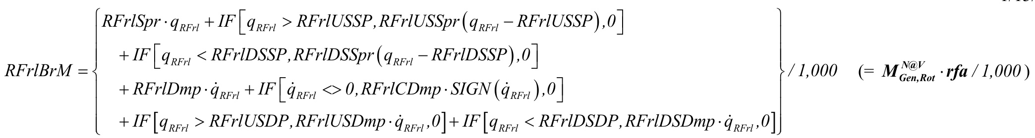
RFrlBrM=MGNe@n,VRo ⋅rfa/ 1,000

Rotor-furl bearing furl moment (about the rotor-furl axis), (\mathrm{kN\cdotm})

Like the LSShftTq and LSSTipMza, it is noted that the rotor-furling furl moment can be computed differently using the rotor-furl springs and dampers, though the load summation method and this other constraint method are equivalent. This can be demonstrated as follows. First of all, the equation above is equivalent to saying:

R F r l B r M=}^{E}\omega_{R F r l}^{R}\cdot M_{G e n,R o t}^{N@V}/{I,O O O}

Or,

RFrlBrM =^{E}\omega_{R F r}^{R}\cdot\Bigg[M_{R o t o r}^{L@P}+\boldsymbol{r}^{V P}\times\boldsymbol{F}_{R o t o r}^{P}-m^{R}\boldsymbol{r}^{V D}\times\left(^{E}\boldsymbol{a}^{D}+g\boldsymbol{z}_{2}\right)-\overline{{\boldsymbol{I}}}^{R}\cdot^{E}\boldsymbol{a}^{R}-^{E}\omega^{R}\times\overline{{\boldsymbol{I}}}^{R}\cdot^{E}\boldsymbol{\omega}^{R}-^{E}\boldsymbol{a}^{R}\cdot^{E}\boldsymbol{a}^{R}\Bigg], IG⋅EαG−EωG×IG⋅EωG/ 1,000

Now applying the cyclic permutation law of the scalar triple product:

=\left[\begin{array}{l}{{\varepsilon_{\omega_{R F H}^{R}}\times r^{V P}\cdot F_{R o t o r}^{P}-m^{R}\,\varepsilon_{\omega_{R F H}^{R}}\times r^{V D}\cdot\left({\varepsilon_{a}}^{P}+{g}{z_{2}}\right)}}\\ {{\;+\;{^{E}\omega}_{R F H}^{R}\cdot\left(M_{R o t o r}^{L@P}-\overline{{{I}}}^{R}\cdot{^{E}{\alpha}^{R}}-{^{E}{\omega}^{R}}\times\overline{{{I}}}^{R}\cdot{^{E}{\omega}^{R}}-\overline{{{I}}}^{G}\cdot{^{E}{\alpha}^{G}}-{^{E}{\omega}^{G}}\times\overline{{{I}}}^{G}\cdot{^{E}{\omega}^{G}}\right)\right]/\left[\begin{array}{l}{{\varepsilon_{a}}^{R}}\\ {{\varepsilon_{b}}^{R}}\end{array}\right]}}\end{array}

Recognizing also that {}^{E}{\nu}_{R F r l}^{P}={}^{E}{\omega}_{R F r l}^{R}\times{r}^{V P} and {}^{E}{\nu}_{R F r l}^{D}={}^{E}{\omega}_{R F r l}^{R}\times{r}^{V D} , and also that ^E{\pmb{\omega}}_{R F r l}^{L}\,,\ {^E\pmb{\omega}}_{R F r l}^{R} , and ^E_{\omega_{R F r l}^{G}} , are equal, this can be expanded as follows:

B r M=\left[{}^{E}\nu_{R F r i}^{P}\cdot F_{R o t o r}^{P}+{}^{E}\omega_{R F r i}^{L}\cdot M_{R o t o r}^{L@P}-m^{R\ E}\nu_{R F r i}^{D}\cdot\left({}^{E}a^{D}+g z_{2}\right)-{}^{E}\omega_{R F r i}^{R}\cdot\left({\overline{{{I}}}}^{R}\cdot{}^{E}a^{R}+g z_{1}\right)\right].

^{R\;E}\nu_{R F H}^{\;D}\cdot\left(^{E}a^{D}+g\bar{z}_{2}\right)-^{E}\omega_{R F H}^{R}\cdot\left(\overline{{{\overline{{{I}}}}}}\bar{}^{R}\cdot^{E}a^{R}+^{E}\omega^{R}\times\overline{{{\overline{{{I}}}}}}^{R}\cdot^{E}\omega^{R}\right)-^{E}\omega_{R F H}^{G}\cdot\left(\overline{{{\overline{{{I}}}}}}\bar{}^{G}\cdot^{E}a^{G}+^{E}\omega^{R}\times\overline{{{\overline{{{I}}}}}}\omega^{R}\right)

\begin{array}{l}{{F_{R F r l}}{\Big|}_{R o t o r}+{F_{R F r l}^{*}}{\Big|}_{R}+{F_{R F r l}}{\Big|}_{G r a v R}+{F_{R F r l}^{*}}{\Big|}_{G}\Big)\thinspace/\thinspace I,000}\\ {\mathrm{~}}\\ {{F_{R F r l}^{*}}{\Big|}_{R}+{F_{R F r l}^{*}}{\Big|}_{H}+{F_{R F r l}^{*}}{\Big|}_{B I}+{F_{R F r l}^{*}}{\Big|}_{B2}+{F_{R F r l}^{*}}{\Big|}_{G}+{F_{R F r l}}{\Big|}_{A e r o B I}+{F_{R F r l}}{\Big|}_{A e r o B2}+{F_{R F r l}}{\Big|}_{G r a v R}+{F_{R F l}}{\Big|}_{G r a v R}+{F_{R F r l}}}\end{array}

\left.\gamma\right|_{G}+F_{R F r}\right|_{A e r o B I}+F_{R F r}\right|_{A e r o B2}+F_{R F r}\right|_{G r a v e}+F_{R F r}\right|_{G r a v e H}+F_{R F r}\right|_{G r a v e B I}+F_{R F r}\right|_{G r a v e B I}=F_{R F r}\Big|_{G r a v e B2}\Big//\left.I,000

From the equations of motion, it is easily seen that this is equivalent to saying:

R F r l B r M=\left(-\left.F_{R F r l}\right|_{S p r i n g R F}-\left.F_{R F r l}\right|_{D a m p R F}\right)/\,l,000

and thus,

Thus, both the load summation method and the constraint method are equivalent. Thus, to avoid using 2 different methods to calculate RFrlBrM if various DOFs are disabled, it is best just to use M_{G e n,R o t}^{N@V}\cdot r\mathbf{f}a\left/I,O O O\right. , which will always work.

Tail-Furl Axis Loads:

There is 1 output load on the tail-furl axis. This is the tail-furl moment about the tail-furl axis. Of course, we could also output all 6 components of the force F_{T a i l}^{\mu} / moment M_{T a i l}^{N\!\alpha\mu} acting on the tail-furl axis at point W on the nacelle. Following the analysis for finding the rotor-furl loads, the new generalized active force for the equations of motion resulting from these new loads is:

F_{r}|_{T a i l}={^{E}\nu_{r}^{W}}\cdot F_{T a i l}^{W}+{^{E}\omega_{r}^{N}}\cdot M_{T a i l}^{N\overline{{{\omega}}}W}\quad\left(r=I,2,...,22\right)

This generalized active force must produce the same effects as the generalized active and inertia forces associated with the tail and tail fin. Thus,

F_{r}|_{T a i l}=F_{r}^{*}|_{A}+F_{r}|_{G r a v d}+F_{r}|_{A e r o A}+F_{r}|_{S p r i n g T F}+F_{r}|_{D a m p T F}\quad(r=I,2,\dots,22)

Since ^E_{\nu_{r}^{\mu}} and ^E\pmb{\omega}_{r}^{N} are equal to zero unless r=1,2,...,11 , the generalized active forces associated with tail-furl elasticity and damping do not contribute to the tail-furl loads (since also, F_{r}|_{S p r i n g T F} and F_{r}|_{D a m p T F} are equal to zero if r\!=\!1,\!2 ,…,11). So,

F_{r}\big|_{T a i l}=F_{r}^{*}\big|_{A}+F_{r}\big|_{G r a v A}+F_{r}\big|_{A e r o A}\quad\big(r=I,2,...,I I\big)

Thus,

{\v{r}}_{I}=-m^{B\ E}\nu_{\nu_{r}}^{I}\cdot\left({\v{\overline{{\varepsilon}}}}_{a}^{\ E}+g\Xi_{2}\right)-m^{F\ E}\nu_{\nu_{r}}^{J}\cdot\left({\v{\overline{{\varepsilon}}}}_{a}^{\ E}+g\Xi_{2}\right)+{\v{}}^{E}\nu_{r}^{K}\cdot F_{A e r o t}^{K}+{\v{}}^{E}\omega_{r}^{A\cdot}\cdot\left(M_{A e r o t}^{A\quad}-\overline{{{\bar{I}}}}^{\ A}\cdot F_{A e r o t}^{B\quad}\right),

However, ^E{\omega}_{r}^{A} and ^E{\pmb\omega}_{r}^{N} are all equal when r is con \begin{array}{r}{^{E}\nu_{r}^{J}={}^{E}\nu_{r}^{W}+{}^{E}\omega_{r}^{N}\times{r}^{W J}\,,\qquad\mathrm{and}\qquad^{E}\nu_{r}^{K}={}^{E}\nu_{r}^{W}+{}^{E}\omega_{r}^{N}\times{r}^{W K}\,,}\end{array} when r=1,2,...,11 , this generalized force can be expanded to:

\begin{array}{r l}&{+\phantom{}^{E}\nu_{r}^{K}\cdot F_{A e r o A}^{K}+\phantom{}^{E}\omega_{r}^{A}\cdot\left(M_{A e r o A}^{A}-\overline{{\overline{{I}}}}\,^{A}\cdot{}^{E}\alpha^{A}+{}^{E}\omega^{A}\times\overline{{\overline{{I}}}}\,^{A}\cdot{}^{E}\omega^{A}\right)\quad\left(r=I,2,\ldots,I I\right)}\\ &{\mathrm{strained~to~be~between~1~and~11.~Recognizing~also~that}\qquad\phantom{.}^{E}\nu_{r}^{I}={}^{E}\nu_{r}^{W}+{}^{E}\omega_{r}^{N}\times{}r^{W I}}\end{array}

\begin{array}{r l}&{\_=\Big(^{E}\pmb{\nu}_{r}^{W}+^{E}\omega_{r}^{N}\times\pmb{r}^{W K}\Big)\cdot\pmb{F}_{\_{A e r o A}}^{K}-m^{B}\left(^{E}\nu_{r}^{W}+^{E}\omega_{r}^{N}\times\pmb{r}^{W I}\right)\cdot\left(^{E}\pmb{a}^{I}+g\Xi_{2}\right)-m^{F}\left(^{E}\nu_{r}^{W}+^{E}\omega_{r}^{A}\times^{A}\right)}\\ &{\quad+\;^{E}\omega_{r}^{N}\cdot\left(\pmb{M}_{\_{A e r o A}}^{A}-\overline{{\overline{{I}}}}\cdot^{A}\cdot^{E}\alpha^{A}-^{E}\omega^{A}\times\overline{{\overline{{I}}}}\mathcal{A}\cdot^{E}\omega^{A}\right)}\end{array}

Now applying the cyclic permutation law of the scalar triple product:

\begin{array}{r l}&{\mathbf{\nabla}_{r}^{\mathcal{W}}\cdot\left[F_{A e r o A}^{K}-m^{B}\left(\mathbf{\nabla}^{E}a^{I}+g z_{2}\right)-m^{F}\left(\mathbf{\nabla}^{E}a^{J}+g z_{2}\right)\right]}\\ &{+\mathbf{\nabla}^{E}\omega_{r}^{N}\cdot\left(M_{A e r o A}^{A}+r^{\mathcal{W}K}\times F_{A e r o A}^{K}-m^{B}r^{\mathcal{W}I}\times\left(\mathbf{\nabla}^{E}a^{I}+g z_{2}\right)-m^{F}r^{\mathcal{W}J}\times\left(\mathbf{\mathcal{E}}a^{J}+g z_{2}\right)-\overline{{\mathbf{\nabla}}}^{A}\cdot\mathbf{\nabla}^{E}a^{J}\right),}\end{array}

Thus it is seen that,

\begin{array}{l}{{\displaystyle-m^{B}\left({\vphantom{\int}}^{E}a^{I}+g z_{2}\right)-m^{F}\left({\vphantom{\int}}^{E}a^{J}+g z_{2}\right)}}\\ {{\displaystyle}}\\ {{\displaystyle-m^{A}+r^{W\kappa}\times{\cal F}_{A e n d}^{\kappa}-m^{B}r^{W}\times\left({\vphantom{\int}}^{E}a^{I}+g z_{2}\right)-m^{F}r^{W\kappa}\times\left({\vphantom{\int}}^{E}a^{J}+g z_{2}\right)-\overline{{\overline{{I}}}}^{A}\cdot{\vphantom{\int}}\alpha^{A}-{\vphantom{\int}}_{\omega}^{4}\omega^{4}\times\overline{{\overline{{I}}}}^{J}\times\left(-g z_{2}\right)}}\\ {{\displaystyle}}\\ {{\displaystyle-m^{B}\left\{\left(\sum_{i=I}^{I}E_{\nu_{i}^{I}}{\vphantom{\int}}^{\vec{\dagger}}\vec{q}_{i}\right)+{\vphantom{\int}}^{E}{\nu}_{T r{\vec{U}}}^{I}{\ddot{q}}_{T r i}\right.+\left[\sum_{i=d}^{I}\frac{d}{d t}\left({\vphantom{\int}}^{\varepsilon}\nu_{i}^{I}\right){\dot{q}}_{i}\right]+\frac{d}{d t}\left({\vphantom{\int}}^{\varepsilon}\nu_{T r{\vec{U}}}^{I}\right){\dot{q}}_{T r i}+g z_{2}\right\}}}\\ {{\displaystyle}}\\ {{\displaystyle-m^{F}\left\{\left(\sum_{i=I}^{I}\varepsilon_{\nu_{i}^{\prime}}{\vec{q}}_{i}\right)+{\vphantom{\int}}^{E}{\nu}_{T r{\vec{U}}}^{J}{\ddot{q}}_{T r i}+\left[\sum_{i=d}^{I}\frac{d}{d t}\left({\vphantom{\int}}^{\varepsilon}\nu_{i}^{\prime}\right){\dot{q}}_{i}\right]+\frac{d}{d t}\left({\vphantom{\cal F}}_{\nu T r}^{J}\right){\dot{q}}_{T r i}+g z_{2}\right\}}}\end{array}

\begin{array}{c}{{\displaystyle r_{T a l}^{N\alpha W}=M_{~A e r o A}^{4}+r^{W K}\times F_{_{A e r o A}}^{K}-m^{B}r^{W}\times\left\{\left(\displaystyle\sum_{i=I}^{I I}\varepsilon_{\nu_{i}^{I}}\ddot{q}_{i}\right)+{}^{E}\nu_{T e r i}^{I}\ddot{q}_{T r r i}+\left[\displaystyle\sum_{i=I}^{I I}\frac{d}{d t}\Big({}^{E}\nu_{{\nu}_{i}^{I}}^{I}\Big)\dot{q}_{i}\right]+:}}\\ {{\displaystyle-m^{F}r^{W J}\times\left\{\left(\displaystyle\sum_{i=I}^{I I}\varepsilon_{\nu_{i}^{J}}\ddot{q}_{i}\right)+{}^{E}\nu_{T e r i}^{J}\ddot{q}_{T r r i}+\left[\displaystyle\sum_{i=I}^{I I}\frac{d}{d t}\Big({}^{E}\nu_{{\nu}_{i}^{J}}^{J}\Big)\dot{q}_{i}\right]+\frac{d}{d t}\Big({}^{E}\nu_{T r r i}^{J}\Big)\dot{q}_{T r r i}+g z_{i},}}\\ {{\displaystyle-\overline{{\bar{I}}}^{\,4}\cdot\left\{\left(\displaystyle\sum_{i=I}^{I I}\varepsilon_{\omega_{i}^{A}}\ddot{q}_{i}\right)+{}^{E}\omega_{T r r i}^{A}\ddot{q}_{T r r i}+\left[\displaystyle\sum_{i=I}^{I I}\frac{d}{d t}\Big({}^{E}\omega_{i}^{A}\Big)\dot{q}_{i}\right]+\frac{d}{d t}\Big({}^{E}\omega_{T r r i}^{A}\Big)\dot{q}_{T r r i}\Big\}-{}^{E}\omega_{T r i}^{J}\;,}}\end{array}

Or,

\begin{array}{l}{{\displaystyle F_{r a i_{r}}^{\scriptscriptstyle{W}}=-m^{B}\,^{\cal E}{}_{\nu}^{\scriptscriptstyle{E}}-m^{\cal F}\,^{\scriptscriptstyle{E}}\nu_{\nu}^{\scriptscriptstyle{J}}\quad\left(r=l,2,\ldots,l{l};l5\right)\nonumber}}\\ {{\displaystyle F_{r a i_{t}}^{\scriptscriptstyle{W}}=F_{\scriptscriptstyle{A e r o}}^{\scriptscriptstyle{K}}-m^{B}\,\biggl\{\biggl[\sum_{i=d}^{\underline{{{l}}}}\frac{d}{d t}\Bigl(^{\varepsilon}\nu_{i}^{\prime}\Bigr)\dot{q}_{i}\biggr]+\frac{d}{d t}\Bigl(^{\varepsilon}\nu_{\scriptscriptstyle{F H}}^{\prime}\Bigr)\dot{q}_{\scriptscriptstyle{T F r l}}+g z_{2}\biggr\}-m^{\cal F}\,\biggl\{\biggl[\sum_{i=d}^{\underline{{{l}}}}\frac{d}{d t}\Bigl(^{\varepsilon}\nu_{i}^{\prime}\Bigr)\dot{q}_{i}\biggr]\nonumber}}\end{array} +ddt(EvTJFrl)qTFrl+gz2
and
MTNai@lrW \begin{array}{l}{{\displaystyle-m^{B}r^{W I}\times^{E}\nu_{r}^{I}-m^{F}r^{W J}\times^{E}\nu_{r}^{J}-\overline{{{\bar{I}}}}{^{A}}\cdot^{E}\omega_{r}^{A}}}&{{\left(r=I,2,\ldots,I I;I5\right)}}\\ {{\displaystyle M_{_{A e r o A}}^{4}+r^{W K}\times F_{_{A e r o A}}^{K}-m^{B}r^{W J}\times\left\{\left[\sum_{i=4}^{I I}\frac{d}{d t}\Big(^{E}\nu_{i}^{I}\Big)\dot{q}_{i}\right]+\frac{d}{d t}\Big(^{E}\nu_{_{T R I}}^{I}\Big)\dot{q}_{T e r t}+g z_{2}\Bigg\}-m^{F}r^{W J}\times\left\{\begin{array}{l}{{\displaystyle-m^{B}}}\\ {{\displaystyle-\frac{1}{d t}\Big(^{E}\omega_{_{I}}^{A}\Big)\dot{q}_{T e r t}\Bigg\}-^{E}\omega^{A}\times\overline{{{\bar{I}}}}{^{A}}\cdot^{E}\omega^{A}}}\end{array}\right.}}\\ {{\displaystyle-\,\overline{{{\bar{I}}}}^{A}\cdot\left\{\sum_{i=7}^{I I}\frac{d}{d t}\Big(^{E}\omega_{i}^{A}\Big)\dot{q}_{i}\right\}+\frac{d}{d t}\Big(^{E}\omega_{_{T F I}}^{A}\Big)\dot{q}_{T e r t}\Bigg\}-^{E}\omega^{A}\times\overline{{{\bar{I}}}}^{A}\cdot^{E}\omega^{A}}}\end{array}
M t TNai@lW = ∑ddt(EviJ)qi+ddt(EvTJFrl)qTFrl+gz2

The output loads is as follows,

TFrlBrM=MTNai@lW ⋅tfa/ 1,000

Tail-furl bearing furl moment (about the tail-furl axis), (\mathrm{kN}\!\cdot\!\mathrm{m})

Like the LSShftTq, LSSTipMza, and RFrlBrM, it is noted that the tail-furling furl moment can be computed differently using the tail-furl springs and dampers, though the load summation method and this other constraint method are equivalent. This can be demonstrated as follows. First of all, the equation above is equivalent to saying:

T F r l B r M=\mathit{\Omega}^{E}\omega_{T F r l}^{A}\cdot M_{T a i l}^{N\ @W}\mathit{\Omega}/\mathit{I},000

Or, TFrlBrM =^{E}\omega_{T H}^{A}\cdot\left[M_{A e r o A}^{A}+r^{W K}\times F_{A e r o A}^{K}-m^{B}r^{W I}\times\left(^{E}a^{I}+g z_{2}\right)-m^{F}r^{W J}\times\left(^{E}a^{J}+g z_{2}\right)-\overline{{{\overline{{{I}}}}}}^{A}\cdot^{E}\omega_{S}\right] αA−EωA×IA⋅EωA/ 1,000

Now applying the cyclic permutation law of the scalar triple product:

\begin{array}{r l}&{^{E}\omega_{T F r i}^{A}\times r^{W\kappa}\cdot F_{^{A_{e r o d.}}}^{K}-m^{B\;E}\omega_{T F r i}^{A}\times r^{W H}\cdot\left(^{E}a^{I}+g z_{2}\right)-m^{F\;E}\omega_{T F r i}^{A}\times r^{W J}\cdot\left(^{E}a^{J}+g z_{2}\right)\Biggr]/I_{^{\prime}F r i}}\\ &{\quad+\;^{E}\omega_{T F r i}^{A}\cdot\left(M_{^{A_{e r o d.}}}^{A}-\overline{{\overline{{I}}}}^{\;a}\cdot^{E}\alpha^{A}-^{E}\omega^{A}\times\overline{{\overline{{I}}}}^{\;a}\cdot^{E}\omega^{A}\right)}\end{array}

Recognizing also that {}^{E}\nu_{T F r l}^{I}={}^{E}\omega_{T F r l}^{A}\times r^{W I} {}^{E}\nu_{T F r l}^{J}={}^{E}\omega_{T F r l}^{A}\times r^{W J} , and {}^{E}\nu_{T F r l}^{K}={}^{E}\omega_{T F r l}^{A}\times r^{W K} , this can be expanded as follows:

T F r/B r M=\left[{\ \varepsilon_{\nu_{T H r M}}^{\kappa}\cdot F_{A e r o A}^{\kappa}+\varepsilon_{\omega_{T H r i}^{A}}^{\kappa}\cdot M_{A e r o A}^{A}-m^{B\;E}\nu_{\nu_{T H}}^{I}\cdot\left({\varepsilon_{a}^{I}}+{\varepsilon_{\bar{z}}}_{2}\right)-m^{F\;E}\nu_{T H}^{J}\cdot\left({\varepsilon_{a}^{A}}+{\varepsilon_{b}}\right)}\right]. _{\!\gamma}\cdot\left(^{\varepsilon}a^{I}+g z_{2}\right)-m^{F~E}\nu_{_{I F H}}^{J}\cdot\left(^{E}a^{J}+g z_{2}\right)-^{\varepsilon}\omega_{_{I F H}}^{A}\cdot\left(\overline{{{I}}}^{\,4}\cdot^{E}\alpha^{4}+^{E}\omega^{A}\times\overline{{{I}}}^{\,4}\cdot^{E}\omega^{A}\right)\right]/I,00 0
or,
T F r l B r M=\left(F_{T F r l}^{*}\vert_{A}+F_{T F r l}\vert_{G r a v A}+F_{T F r l}\vert_{A e r o A}\right)/\,I,000

From the equations of motion, it is easily seen that this is equivalent to saying:

T F r l B r M=\left(-\left.F_{T F r l}\right\vert_{S p r i n g T F}-F_{T F r l}\right\vert_{D a m p T F}\right)/\left.I,000

and thus,

M=\left\{\begin{array}{l l}{{T F r l S p r cdot q_{T r r l}+I F\left[q_{T r r l}>T F r/U S S P,T F r/U S S p r\left(q_{T r r l}-T F r/U S S P\right),0\right]}}\\ {{+I F\left[q_{T r l}<T F r/D S S P,T F r/D S S p r\left(q_{T r r l}-T F r/D S S P\right),0\right]}}\\ {{+T F r/D m p\cdot\dot{q}_{T r r l}+I F\left[\dot{q}_{T r r l}\gg0,T F r/C D m p\cdot S I G N\left(\dot{q}_{T r r l}\right),0\right]}}\\ {{+I F\left[q_{T r l}>T F r/U S D P,T F r/U S D m p\cdot\dot{q}_{T r r l},0\right]+I F\left[q_{T r l}<T F r/D S D P,T F r/D F\right]}}\end{array}\right.

Thus, both the load summation method and the constraint method are equivalent. Thus, to avoid using 2 different methods to calculate TFrlBrM if various DOFs are disabled, it is best just to use M_{T a i l}^{N@W}\cdot t\mathbf{f}\mathbf{a}\,/\,I,O O O , which will always work.

Tower Top / Yaw Bearing Loads:

There are 10 output loads at the tower top / yaw bearing location. 5 of them are the 3 components of tower top force F_{N a c,R o t}^{o} (2 components are expressed in a nonrotating frame, 2 components are expressed in a rotating frame, and 1 component is independent of rotation). The 5 other loads are the 3 components of the tower top bending moment, M_{N a c,R o t}^{B@O} (again, 2 components are expressed in a nonrotating frame, 2 components are expressed in a rotating frame, and 1 component is independent of rotation). All these loads are given relative to point O as indicated. Note that none of these loads include the effects of the yaw bearing mass (YawBrMass), which would affect the forces but not the moments. The new generalized active force for the equations of motion resulting from these new loads is:

在塔顶/偏航承载位置有10个输出负载。其中5个是塔顶力的3个分量$F_{N a c,R o t}^{o}$ （2个分量以非旋转框架表示，2个分量以旋转框架表示，1个分量与旋转无关）。另外5个负载是塔顶弯矩的3个分量  M_{N a c,R o t}^{B@O} （同样，2个分量以非旋转框架表示，2个分量以旋转框架表示，1个分量与旋转无关）。所有这些负载相对于点 O 给出。请注意，这些负载不包括偏航承载质量（YawBrMass）的影响，后者会影响力但不影响矩。由于这些新负载导致运动方程中的新广义活动力为：

F_{r}\big|_{N a c,R o t}={^{E}\nu_{r}^{o}}\cdot F_{N a c,R o t}^{o}+{^{E}\omega_{r}^{B}}\cdot M_{N a c,R o t}^{B@O}\quad\left(r=1,2,...,22\right)

This generalized active force must produce the same effects as the generalized active and inertia forces associated with everything but the tower and platform. Thus,

\begin{aligned}
\left.F_r\right|_{\text {Nac,Rot }}= & \left.\left.F_r^*\right|_N +F_r^*\right|_R+\left.F_r^*\right|_G+\left.F_r^*\right|_H+\left.F_r^*\right|_{\text {B1 }}+\left.\left.F_r^*\right|_{B 2} F_r^*\right|_A \\
& +\left.F_r\right|_{\text {AeroB1 }}+\left.F_r\right|_{\text {AeroB2 }}+\left.F_r\right|_{\text {AeroA }}+\left.F_r\right|_{\text {GravN }}+\left.F_r\right|_{\text {GravR }}+\left.F_r\right|_{\text {GravH }}+\left.F_r\right|_{\text {GravB1 }}+\left.F_r\right|_{\text {GravB2 }}+\left.F_r\right|_{\text {GravA }}+\left.F_r\right|_{\text {Gen }}+\left.F_r\right|_{\text {Brake }}+\left.F_r\right|_{\text {GBFric }} \quad(r=1,2, \ldots, 22) \\
& +\left.F_r\right|_{\text {SpringYaw }}+\left.F_r\right|_{\text {DampYaw }}+\left.F_r\right|_{\text {SpringRF }}+\left.F_r\right|_{\text {DampRF }}+\left.F_r\right|_{\text {SpringTeet }}+\left.F_r\right|_{\text {DampTeet }}+\left.F_r\right|_{\text {SpringTF }}+\left.F_r\right|_{\text {DampTF }} \\
& +\left.F_r\right|_{\text {ElasticB1 }}+\left.F_r\right|_{\text {DampB1 }}+\left.F_r\right|_{\text {ElasticB } 2}+\left.F_r\right|_{\text {DampB } 2}+\left.F_r\right|_{\text {ElasticDrive }}+\left.F_r\right|_{\text {DampDrive }}
\end{aligned}

Since {^{E}\nu_{r}^{o}} and {^{E}\omega_{r}^{B}} are equal to zero unless r=1,2,...,10 , the generalized active forces associated with blade, drivetrain, yaw, rotor-furl, tail-furl, and teeter elasticity and damping as well as the generator torque, high-speed shaft braking torque, and gearbox friction do not contribute to the tower top loads (since also, F_r^*|_{ElasticB1}, F_r^*|_{DampB1}, F_r^*|_{ElasticB2} \left.\phantom{\frac{1}{\mu_{2}}}\!\!\!,F\right|_{D a m p B2},\left.F\right|_{S p r i n g T e e},\left.F\right|_{D a m p T e e},\left.F\right|_{S p r i n g R F},\left.F\right|_{D a m p R F},\left.F\right|_{S p r i n g T e},\left.F\right|_{D a m p T e},\left.F\right|_{D a m p T e},\left.F\right|_{D a m p T e},\left.F\right|_{P a n p T e} SpringYaw, Fr DampYaw, F_{r}|_{E l a s t i c D r i v e}\,,\;F_{r}|_{D a m p D r i v e}\,,\;F_{r}|_{G e n}\,,\;F_{r}|_{B r a k e}\,; , and F_{r}|_{G B F r i c} are equal to zero if r=1,2,...,10\rangle ). So,

\begin{aligned}
\left.F_r\right|_{\text {Nac,Rot }} & =\left.F_r^*\right|_{B 1}+\left.F_r\right|_{\text {AeroB1 }}+\left.F_r\right|_{G r a v B 1}+\left.F_r^*\right|_{B 2}+\left.F_r\right|_{\text {AeroB } 2}+\left.F_r\right|_{G r a v B 2}+\left.F_r^*\right|_H+\left.F_r\right|_{G r a v H}+\left.F_r^*\right|_R+\left.F_r\right|_{G r a v R}+\left.F_r^*\right|_G \quad(r=1,2, \ldots, 10) \\
& +\left.F_r^*\right|_A+\left.F_r\right|_{G r a v A}+\left.F_r\right|_{\text {AeroA }}+\left.F_r^*\right|_N+\left.F_r\right|_{G r a v N}
\end{aligned}

When using the results for the rotor-furl and tail-furl loads, this equation can be simplified as follows:

F_{r}\big|_{N a c,R o t}=F_{r}\big|_{G e n,R o t}+F_{r}\big|_{T a i l}+F_{r}^{*}\big|_{N}+F_{r}\big|_{G r a v N}\quad\big(r=I,2,\dots,I0\big)

Thus,

\left.F_r\right|_{\text {Nac,Rot }}={ }^E \boldsymbol{v}_r^V \cdot \boldsymbol{F}_{G e l, R o t}^V+{ }^E \boldsymbol{\omega}_r^N \cdot \boldsymbol{M}_{G e n, \text { Rot }}^{N @ V}+{ }^E \boldsymbol{v}_r^W \cdot \boldsymbol{F}_{\text {Tail }}^W+{ }^E \boldsymbol{\omega}_r^N \cdot \boldsymbol{M}_{\text {Tail }}^{N @ W}-m^{N E} \boldsymbol{v}_r^U \cdot\left({ }^E \boldsymbol{a}^U+g \boldsymbol{z}_2\right)-{ }^E \boldsymbol{\omega}_r^N \cdot\left(\overline{\overline{\boldsymbol{I}}}^N \cdot{ }^E \boldsymbol{\alpha}^N+{ }^E \boldsymbol{\omega}^{\boldsymbol{N}} \times \overline{\overline{\boldsymbol{I}}}^N \cdot{ }^E \boldsymbol{\omega}^{\boldsymbol{N}}\right) \quad(r=1,2, \ldots, 10)

However, ^E\pmb{\omega}_{r}^{N} and ^E{\omega}_{r}^{B} are all equal when r is constrained to be between 1 and 10. Thus, when grouping like terms:

\left.F_r\right|_{\text {Nac,Rot }}={ }^E \boldsymbol{v}_r^V \cdot \boldsymbol{F}_{G e n, R o t}^{\boldsymbol{V}}+{ }^E \boldsymbol{v}_r^W \cdot \boldsymbol{F}_{\text {Tail }}^W-m^{N E} \boldsymbol{v}_r^U \cdot\left({ }^E \boldsymbol{a}^U+g z_2\right)+{ }^E \boldsymbol{\omega}_r^B \cdot\left(\boldsymbol{M}_{G e r, R o t}^{N @ V}+\boldsymbol{M}_{\text {Tail }}^{N @ W}-\overline{\overline{\boldsymbol{I}}}^N \cdot{ }^E \boldsymbol{\alpha}^N-{ }^E \boldsymbol{\omega}^N \times \overline{\overline{\boldsymbol{I}}}^N \cdot{ }^E \boldsymbol{\omega}^N\right) \quad(r=1,2, \ldots, 10)

Recognizing also that { }^E v_r^U={ }^E v_r^O+{ }^E \omega_r^B \times r^{O U} , { }^E v_r^V={ }^E v_r^O+{ }^E \omega_r^B \times r^{O V} , { }^E v_r^W={ }^E v_r^O+{ }^E \omega_r^B \times r^{O W}, when \begin{array}{r l r}{r}&{{}=}&{1,2,...,10,}\end{array} , this generalized force can be expanded to:

\begin{aligned}
\left.F_r\right|_{\text {Nac, Rot }}= & \left({ }^E \boldsymbol{v}_r^o+{ }^E \boldsymbol{\omega}_r^B \times \boldsymbol{r}^{O \boldsymbol{V}}\right) \cdot \boldsymbol{F}_{\text {Gen,Rot }}^V+\left({ }^E \boldsymbol{v}_r^O+{ }^E \boldsymbol{\omega}_r^B \times \boldsymbol{r}^{O W}\right) \cdot \boldsymbol{F}_{\text {Tail }}^W-m^N\left({ }^E \boldsymbol{v}_r^O+{ }^E \boldsymbol{\omega}_r^B \times \boldsymbol{r}^{O U}\right) \cdot\left({ }^E \boldsymbol{a}^U+g \boldsymbol{z}_2\right) \\
& +{ }^E \boldsymbol{\omega}_r^B \cdot\left(\boldsymbol{M}_{\text {Gen,Rot }}^{N @ V}+\boldsymbol{M}_{\text {Tail }}^{N @ W}-\overline{\overline{\boldsymbol{I}}}^N \cdot{ }^E \alpha^N-{ }^E \boldsymbol{\omega}^N \times \overline{\overline{\boldsymbol{I}}}^N \cdot{ }^E \boldsymbol{\omega}^N\right)
\end{aligned}

Now applying the cyclic permutation law of the scalar triple product:

\begin{aligned}
\left.F_r\right|_{\text {Nac,Rot }}= & { }^E \boldsymbol{v}_r^O \cdot\left[\boldsymbol{F}_{\text {Geln,Rot }}^V+\boldsymbol{F}_{\text {Tail }}^W-m^N\left({ }^E \boldsymbol{a}^U+g \boldsymbol{z}_2\right)\right]+{ }^E \boldsymbol{\omega}_r^B \cdot\left[r^{O \boldsymbol{V}} \times \boldsymbol{F}_{\text {Gel, Rot }}^V+r^{\boldsymbol{OW}} \times \boldsymbol{F}_{\text {Tail }}^W-m^N r^{O U} \times\left({ }^E \boldsymbol{a}^U+g z_2\right)\right] \quad(r=1,2, \ldots, 10) \\
& +{ }^E \boldsymbol{\omega}_r^B \cdot\left(\boldsymbol{M}_{\text {Geln,Rot }}^{N @ V}+\boldsymbol{M}_{\text {Tail }}^{N @W}-\overline{\overline{\boldsymbol{I}}}^N \cdot{ }^E \boldsymbol{\alpha}^N-{ }^E \boldsymbol{\omega}^N \times \overline{\overline{\boldsymbol{I}}}^N \cdot{ }^E \boldsymbol{\omega}^N\right)
\end{aligned}

which simplifies to:

\begin{aligned}
\left.F_r\right|_{\text {Nac, Rot }}= & { }^E \boldsymbol{v}_r^O \cdot\left[\boldsymbol{F}_{\text {Gen,Rot }}^V+\boldsymbol{F}_{\text {Tail }}^W-m^N\left({ }^E \boldsymbol{a}^U+g z_2\right)\right] \\
& +{ }^E \boldsymbol{\omega}_r^B \cdot\left[\boldsymbol{M}_{\text {Gen,Rot }}^{N @ V}+\boldsymbol{M}_{\text {Tail }}^{N @ W}+\boldsymbol{r}^{O \boldsymbol{V}} \times \boldsymbol{F}_{\text {Gen,Rot }}^V+\boldsymbol{r}^{O\boldsymbol{W}} \times \boldsymbol{F}_{\text {Tail }}^W-m^N r^{O U} \times\left({ }^E \boldsymbol{a}^U+g \boldsymbol{z}_2\right)-\overline{\overline{\boldsymbol{I}}}^N \cdot{ }^E \boldsymbol{\alpha}^N-{ }^E \boldsymbol{\omega}^N \times \overline{\overline{\boldsymbol{I}}}^N \cdot{ }^E \boldsymbol{\omega}^N\right] \quad(r=1,2, \ldots, 10)
\end{aligned}

Thus it is seen that,

\boldsymbol{F}_{\text {Nac,Rot }}^O=\boldsymbol{F}_{\text {Gen,Rot }}^V+\boldsymbol{F}_{\text {Tail }}^W-m^N\left({ }^E \boldsymbol{a}^U+g \boldsymbol{z}_2\right)

and

\boldsymbol{M}_{\text {Nac,Rot }}^{B @ O}=\boldsymbol{M}_{G e n, R o t}^{N @ V}+\boldsymbol{M}_{\text {Tail }}^{N @ W}+\boldsymbol{r}^{O V} \times \boldsymbol{F}_{G e n, R o t}^V+\boldsymbol{r}^{O W} \times \boldsymbol{F}_{\text {Tail }}^W-m^N r^{O U} \times\left({ }^E a^U+g z_2\right)-\overline{\overline{\boldsymbol{I}}}^N \cdot{ }^E \alpha^N-{ }^E \omega^N \times \overline{\overline{\boldsymbol{I}}}^N \cdot{ }^E \omega^N

Thus,

\boldsymbol{F}_{\text {Nac,Rot }}^o=\boldsymbol{F}_{\text {Gen,Rot }}^{\boldsymbol{V}}+\boldsymbol{F}_{\text {Tail }}^{\boldsymbol{W}}-m^N\left\{\left(\sum_{i=1}^{11}{ }^E \boldsymbol{v}_i^U \ddot{q}_i\right)+\left[\sum_{i=4}^{11} \frac{d}{d t}\left(\boldsymbol{v}^E \boldsymbol{v}_i^U\right) \dot{q}_i\right]+g \boldsymbol{z}_2\right\}

and

\begin{aligned}
& \boldsymbol{M}_{\text {Nac,Rot }}^{\text {B@O }}=\boldsymbol{M}_{\text {Geln,Rot }}^{N @ V}+\boldsymbol{M}_{\text {Tail }}^{\text {N@W }}+\boldsymbol{r}^{O V} \times \boldsymbol{F}_{\text {Gel, Rot }}^V+\boldsymbol{r}^{OW} \times \boldsymbol{F}_{\text {Tail }}^W-m^N r^{O U} \times\left\{\left(\sum_{i=1}^{11}{ }^E \boldsymbol{v}_i^U \ddot{q}_i\right)+\left[\sum_{i=4}^{11} \frac{d}{d t}\left({ }^E \boldsymbol{v}_i^U\right) \dot{q}_i\right]+g z_2\right\} \\
& -\overline{\overline{\boldsymbol{I}}}^N \cdot\left\{\left(\sum_{i=4}^{11}{ }^E \boldsymbol{\omega}_j^N \ddot{q}_i\right)+\left[\sum_{i=7}^{11} \frac{d}{d t}\left({ }^E \boldsymbol{\omega}_i^N\right) \dot{q}_i\right]\right\}-{ }^E \boldsymbol{\omega}^N \times \overline{\overline{\boldsymbol{I}}}^N \cdot{ }^E \boldsymbol{\omega}^N
\end{aligned}

Or,

\begin{array}{l}{{F_{N a c,R o t_{r}}^{o}=F_{G e n,R o t_{r}}^{V}+F_{T a i l_{r}}^{W}-m^{N^{\textit{E}}}\pmb{\nu}_{r}^{U}\quad\left(r=I,2,...,22\right)}}\\ {{\phantom{=}}}\\ {{F_{N a c,R o t_{t}}^{o}=F_{G e n,R o t_{t}}^{V}+F_{T a i l_{t}}^{W}-m^{N}\left\{\left[\sum_{i=4}^{I I}\frac{d}{d t}\!\left(^{\textit{E}}\nu_{i}^{U}\right)\dot{q}_{i}\right]\!\!+g z_{2}\right\}}}\end{array}

and

\boldsymbol{M}_{\text {Nac, Rot }_r}^{B @ O}=\boldsymbol{M}_{G e n, R o t_r}^{\text {N@V }}+\boldsymbol{M}_{\text {Tail }_r}^{N @ W}+\boldsymbol{r}^{O \boldsymbol{V}} \times \boldsymbol{F}_{G e l, R o t_r}^V+\boldsymbol{r}^{O W} \times \boldsymbol{F}_{\text {Tailt}}^W-m^N r^{O U} \times{{ }^E \boldsymbol{v_r}^U} - \overline{\overline{\boldsymbol{I}}}^N \cdot{ }^E \omega_r^N\quad\left(r=I,2,...,22\right)

\boldsymbol{M}_{\text {Nac, Rot }_t}^{B @ O}=\boldsymbol{M}_{G e n, R o t_t}^{\text {N@V }}+\boldsymbol{M}_{\text {Tail }_t}^{N @ W}+\boldsymbol{r}^{o \boldsymbol{V}} \times \boldsymbol{F}_{G e l, R o t_t}^V+\boldsymbol{r}^{O W} \times \boldsymbol{F}_{\text {Tailt}}^W-m^N r^{O U} \times\left\{\left[\sum_{i=4}^{I I} \frac{d}{d t}\left({ }^E \boldsymbol{v}_i^U\right) \dot{q}_i\right]+g z_2\right\}-\overline{\overline{\boldsymbol{I}}}^N \cdot\left[\sum_{i=7}^{I I} \frac{d}{d t}\left({ }^E \boldsymbol{\omega}_i^N\right) \dot{q}_i\right]-{ }^E \boldsymbol{\omega}^N \times \overline{\overline{\boldsymbol{I}}}^N \cdot{ }^E \boldsymbol{\omega}^N

The output loads are as follows,

Y a w B r F x n=F_{N a c,R o t}^{o}\cdot d_{1}\ ⁄1000 Rotating (with nacelle) yaw bearing shear force (directed along the xn-axis), (kN) Y a w B r F y n=-F_{N a c,R o t}^{o}\cdot d_3/1000 Rotating (with nacelle) yaw bearing shear force (directed along the yn-axis), (kN) Y a w B r F x p=F_{N a c,R o t}^{o}\cdot b_{1}/1000 Yaw bearing for-aft (nonrotating) shear force (directed along the xp-axis), (kN) Y a w B r F y p=-F_{N a c,R o t}^{o}\cdot b_{3}/1000 Yaw bearing side-to-side (nonrotating) shear force (directed along the yp-axis), (kN) Y a w B r F z n=Y a w B r F z p=F_{_{N a c,R o t}}^{o}\cdot d_2/1000=F_{_{N a c,R o t}}^{o}\cdot b_2/1000 Yaw bearing axial force (directed along the zn-/zp-axis), (kN) Y a w B r M x n=M_{N a c,R o t}^{B@O}\cdot d_1/1000 Rotating (with nacelle) yaw bearing roll moment (about the xn-axis), \left(\mathrm{kN}\mathrm{\cdot}\mathrm{m}\right)

Y a w B r M y n=M_{N a c,R o t}^{B@O}\cdot d_3/1000 Rotating (with nacelle) yaw bearing pitch moment (about the yn-axis), (kN·m) Y a w B r M x p=M_{N a c,R o t}^{B@O}\cdot b_1/1000 Nonrotating yaw bearing roll moment (about the xp-axis), (kN·m) Y a w B r M y p=-M_{\mathit{N a c},\mathit{R o t}}^{\mathit{B@O}}\cdot b_{3}/1000 Nonrotating yaw bearing pitch moment (about the yp-axis), (kN·m) Y a w B r M z n=Y a w B r M z p=M_{N a c,R o t}^{B@O}\cdot d_2/1000=M_{N a c,R o t}^{B@O}\cdot b_2/1000 Yaw bearing yaw moment (about the zn-/zp-axis), (kN·m)

Like the LSShftTq, LSSTipMza, RFrlBrM, and TFrlBrM, it is noted that the yaw bearing yaw moment can be computed differently using the yaw drive spring and damper, though the load summation method and this other constraint method are equivalent. This can be demonstrated as follows. First of all, the equation above is equivalent to saying:

\text { YawBrMzn }={ }^E \omega_{\text {Yaw }}^N \cdot \boldsymbol{M}_{\text {Nac,Rot }}^{B @ O} / 1,000
$$Or,

\text { YawBrMzn }={ }^E \boldsymbol{\omega}{\text {Yaw }}^N \cdot\left[\boldsymbol{M}{G e n, \text { Rot }}^{N @ V}+\boldsymbol{M}{\text {Tail }}^{N @ W}+\boldsymbol{r}^{O V} \times \boldsymbol{F}{\text {Gen,Rot }}^V+\boldsymbol{r}^{\boldsymbol{O W}} \times \boldsymbol{F}_{\text {Tail }}^{\boldsymbol{W}}-m^N \boldsymbol{r}^{O U} \times\left({ }^E \boldsymbol{a}^U+g \boldsymbol{z}_2\right)-\overline{\overline{\boldsymbol{I}}}^N \cdot{ }^E \boldsymbol{\alpha}^N-{ }^E \boldsymbol{\omega}^N \times \overline{\overline{\boldsymbol{I}}}^N \cdot{ }^E \boldsymbol{\omega}^N\right] / 1,000

Now applying the cyclic permutation law of the scalar triple product:  

\text { YawBrMzn }=\left[\begin{array}{c} { }^E \boldsymbol{\omega}{\text {Yaw }}^N \times \boldsymbol{r}^{\boldsymbol{O V}} \cdot \boldsymbol{F}{\text {Gen,Rot }}^V+{ }^E \boldsymbol{\omega}{\text {Yaw }}^N \times \boldsymbol{r}^{\boldsymbol{O W}} \cdot \boldsymbol{F}{\text {Tail }}^W-m^{N E} \boldsymbol{\omega}{\text {Yaw }}^N \times \boldsymbol{r}^{\boldsymbol{O U}} \cdot\left({ }^E \boldsymbol{a}^U+g \boldsymbol{z}2\right) \ +{ }^E \boldsymbol{\omega}{\text {Yaw }}^N \cdot\left(\boldsymbol{M}{\text {Gen,Rot }}^{\text {NaV }}+\boldsymbol{M}_{\text {Tail }}^{\text {N@W }}-\overline{\overline{\boldsymbol{I}}}^{\boldsymbol{N}} \cdot{ }^E \boldsymbol{\alpha}^{\boldsymbol{N}}-{ }^E \boldsymbol{\omega}^{\boldsymbol{N}} \times \overline{\overline{\boldsymbol{I}}}^N \cdot{ }^E \boldsymbol{\omega}^N\right) \end{array}\right] / 1,000

  

Recognizing also that ${}^{E}{\nu}_{Y a w}^{U}={}^{E}{\omega}_{Y a w}^{N}\times r^{O U}$ ${}^{E}{\nu}_{{\scriptscriptstyle Y a w}}^{V}={}^{E}{\omega}_{{\scriptscriptstyle Y a w}}^{N}\times{r}^{O V}$ and ${}^{E}{\nu}_{Y a w}^{W}={}^{E}{\omega}_{Y a w}^{N}\times r^{O W}$ , this can be expanded as follows:  

$\text { YawBrMzn }=\left[{ }^E \boldsymbol{v}_{\text {Yaw }}^V \cdot \boldsymbol{F}_{\text {Gen,Rot }}^V+{ }^E \boldsymbol{\omega}_{\text {Yaw }}^N \cdot \boldsymbol{M}_{\text {Gen,Rot }}^{\text {NaV }}+{ }^E \boldsymbol{v}_{\text {Yaw }}^W \cdot \boldsymbol{F}_{\text {Tail }}^W+{ }^E \boldsymbol{\omega}_{\text {Yaw }}^N \cdot \boldsymbol{M}_{\text {Tail }}^{\text {N@W }}-m^{N{ }^E} \boldsymbol{v}_{\text {Yaw }}^U \cdot\left({ }^E \boldsymbol{a}^{\boldsymbol{U}}+g \boldsymbol{z}_2\right)-{ }^E \boldsymbol{\omega}_{\text {Yaw }}^N \cdot\left(\overline{\overline{\boldsymbol{I}}}^N \cdot{ }^E \boldsymbol{\alpha}^{\boldsymbol{N}}+{ }^E \boldsymbol{\omega}^{\boldsymbol{N}} \times \overline{\overline{\boldsymbol{I}}}^N \cdot{ }^{\boldsymbol{E}} \boldsymbol{\omega}^{\boldsymbol{N}}\right)\right] / 1,000$
or,   
$\text { YawBrMzn }=\left(\left.F_{\text {Yaw| }}\right|_{\text {Rotor }}+\left.F_{\text {Yaw }}\right|_{\text {Tail }}+\left.F_{\text {Yaw }}^*\right|_N+\left.F_{\text {Yaw}}\right|_{\text {GravN }}\right) / 1,000$  

3r M z n=\left(\begin{array}{c}{F_{Y a w}^{}\Big|{N}+F{Y a w}^{}\Big|{R}+F{Y a w}^{}\Big|{G}+F{Y a w}^{}\Big|{H}+F{Y a w}^{}\Big|{B I}+F{Y a w}^{}\Big|{B2}+F{Y a w}^{}\Big|{A}+F{Y a w}^{}\Big|{A e r o\theta B I}+F{Y a w}}\ {+F_{Y a w}\Big|{G r a v N}+F{Y a w}\Big|{G r a v N}+F{Y a w}\Big|{G r a v H}+F{Y a w}\Big|{G r a v B I}+F{Y a w}\Big|{G r a v B2}+F{Y a w}\Big|_{G r a v B2}}\end{array}\right)

  

From the equations of motion, it is easily seen that this is equivalent to saying:  

\text { YawBrMzn }=\left(-\left.F_{\text {Yav }}\right|{\text {SpringYav }}-\left.F{\text {Yav }}\right|_{\text {DampYavv }}\right) / 1,000

  

and thus,  

 $\text { YawBrMzn }=\left[\operatorname{YawSpr}\left(q_{\text {Yaw }}-\operatorname{YawNeut}\right)+\operatorname{YawDamp} \cdot \dot{q}_{\text {Yav }}\right] / 1,000 \quad\left(=\boldsymbol{M}_{\text {Nac,Rot }}^{\text {B@O }} \cdot \boldsymbol{d}_2 / 1,000\right)$ 

Thus, both the load summation method and the constraint method are equivalent.  Thus, to avoid using 2 different methods to calculate YawBrMzn if various DOFs are disabled, it is best just to use $\boldsymbol{M}_{\mathrm{Nac}, \mathrm{Rot}}^{\mathrm{B@O}} \cdot \boldsymbol{d}_2 / 1,000$ , which will always work.  

# Tower Base Loads:  

There are 6 output loads at the base of the tower.  3 of them are the 3 components of the base force $F_{T u r b}^{T}\left(O\right)$ .  The other 3 are the 3 components of the base bending moments, $M_{T u r b}^{X}\left(O\right)$ .  Note that the tower base loads are all output at the point on the tower where it changes from being rigid to being flexible $(h=0)$ ).  The new generalized active force for the equations of motion resulting from these new loads is:  

F_{r}\big|{T u r b}={^{E}\nu{r}^{T}},\big(0\big)\cdot F_{T u r b}^{T},\big(0\big)+{^{E}\omega_{r}^{X}}\cdot M_{T u r b}^{X},\big(0\big)\quad\big(r=I,2,...,22\big)

  

This generalized active force must produce the same effects as the generalized active and inertia forces associated with everything but the platform. Thus,  

\begin{array}{r l}&{\ddots\bigg|{T}+F{r}^{}\bigg|{N}F{r}^{}\bigg|{R}+F{r}^{}\bigg|{G}+F{r}^{}\bigg|{H}+F{r}^{}\bigg|{B I}+F{r}^{}\bigg|{B I}F{r}^{*}\bigg|{A}}\ &{+F{r}\bigg|{A e r o r}+F{r}\big|{A e r o b I}+F{r}\big|{A e r o b I}+F{r}\big|{A e r o A}+F{r}\big|{G r a v Y}+F{r}\big|{G r a v Y}+F{r}\big|{G r a v Y}+F{r}\big|{G r a v H}+F{r}\big|{G r a v H}}\ &{+F{r}\big|{S p r i a g Y a w}+F{r}\big|{D a m p Y a w}+F{r}\big|{S p r i a g R F}+F{r}\big|{D a m p R F}+F{r}\big|{S p r i a n g T e e t}+F{r}\big|{B a m p T e e t}+F{r}\big|{S p r i a g r T}+F{r}\big|{B r}}\ &{+F{r}\big|{E l a s t i c T}+F{r}\big|{D a m p T}+F{r}\big|{E l a s t i c B I}+F{r}\big|{D a m p B I}+F{r}\big|{E l a s t i c B2}+F{r}\big|{E l a n p B2}+F{r}\big|{E l a s t i c D r i v e}+F{r}\big|_{E l a n g r B v e}}\end{array}

  

Since $\varepsilon_{\nu_{r}^{T}}(\rho)$ and $^E\pmb{\omega}_{r}^{X}$ are equal to zero unless $r=1,2,...,6$ , the generalized active forces associated with blade, drivetrain, yaw, rotor-furl, tail-furl, teeter, and tower  elasticity and damping as well as the generator torque, high-speed shaft braking torque, and gearbox friction do not contribute to the tower base loads (since also, Fr ElasticB1, Fr DampB1, Fr ElasticB2, Fr DampB2, Fr SpringTeet, Fr DampTeet, Fr SpringRF, Fr DampRF, Fr SpringTF, Fr DampTF, Fr SpringYaw, $F_{r}|_{D a m p Y a w}\,,\,F_{r}|_{E l a s t i c D r i v e}\,,\,F_{r}|_{D a m p D r i v e}\,,\,F_{r}|_{G e n}\,,\,F_{r}|_{B r a k e}\,,\,F_{r}|_{G B F r i c}\,,F_{r}|_{E l a s t i c T}\,,$ nd $F_{r}|_{D a m p T}$ are equal to zero if $r=1,2,...,6)$ ).  So,  

FrTurb=F $\begin{array}{r l}&{\overset{*}{\underset{|}{\cdot}}\Big|_{B I}+F_{r}\big|_{A e r o b I}+F_{r}\big|_{G r a v B I}+F_{r}^{*}\Big|_{B2}+F_{r}\big|_{A e r o b2}+F_{r}\big|_{G r a v B2}+F_{r}^{*}\Big|_{H}+F_{r}\big|_{G r a v H}+F_{r}^{*}\Big|_{R}+F_{r}\big|_{G r a v R}+}\\ &{+F_{r}^{*}\Big|_{A}+F_{r}\big|_{G r a v A}+F_{r}\big|_{A e r o d}+F_{r}^{*}\Big|_{N}+F_{r}\big|_{G r a v N}+F_{r}^{*}\Big|_{T}+F_{r}\big|_{A e r o T}+F_{r}\big|_{G r a v T}}\end{array}$ Fr\*G (r=1,2,,6)  

When using the results for the tower-top loads, this equation can be simplified as follows:  

F_{r}\big|{T u r b}=F{r}\big|{N a c,R o t}+F{r}^{*}\big|{T}+F{r}\big|{A e r o T}+F{r}\big|_{G r a v T}\quad\big(r=I,2,...,\theta\big)

  

Thus,  

\begin{array}{r l}{\colon^{E}\nu_{r}^{o}\cdot F_{N a c,R o t}^{o}+^{E}\omega_{r}^{B}\cdot M_{N a c,R o t}^{B\bar{\omega}O}-\overbrace{\int_{\theta}}^{T w r F/e c L}\mu^{T}\left(h\right)^{E}\nu_{r}^{T}\left(h\right)\cdot\left[^{E}a^{T}\left(h\right)+g z_{2}\right]d h-Y a w B r M a t}\ {\uparrow}&{^{T w r F/e c L}}\ {+\overbrace{\int_{\theta}}^{T w r F}\left(\left[h\right)\cdot F_{A e r o r}^{T}\left(h\right)+^{E}\omega_{r}^{F}\left(h\right)\cdot M_{A e r o r}^{F}\left(h\right)\right]d h}\end{array}

  

However, ${}^{E}{\pmb{\omega}}_{r}^{B}\,,\ {}^{E}{\pmb{\omega}}_{r}^{F}\left(h\right)$ , and $^E\pmb{\omega}_{r}^{X}$ are all equal when $r$ is constrained to be between 1 and 6.  Thus,  

\begin{array}{r l}&{:\displaystyle^{E}\nu_{r}^{o}\cdot F_{N a c,R o t}^{o}+^{E}\omega_{r}^{X}\cdot M_{N a c,R o t}^{B@O}-\prod_{\theta}^{T w r F l e c L}\mu^{T}\left(h\right)^{E}\nu_{r}^{T}\left(h\right)\cdot\left[^{E}a^{T}\left(h\right)+g z_{2}\right]d h-Y a w B r M a}\ &{+\displaystyle\int_{0}^{T w r F(h)}\left[^{E}\nu_{r}^{T}\left(h\right)\cdot F_{A e r o r}^{T}\left(h\right)+^{E}\omega_{r}^{X}\left(h\right)\cdot M_{A e r o r}^{F}\left(h\right)\right]d h}\end{array}

  

Recognizing also that $\begin{array}{r}{^{\varepsilon}\nu_{r}^{o}=^{E}\nu_{r}^{r}\left(0\right)+^{E}\omega_{r}^{x}\times\left[r^{z o}-r^{z T}\left(0\right)\right],\qquad\mathrm{and}\qquad^{\varepsilon}\nu_{r}^{r}\left(h\right)=^{\varepsilon}\nu_{r}^{r}\left(0\right)+^{\varepsilon}\omega_{r}^{x}\times\left[r^{z o}-r^{z T}\left(0\right)\right],}\end{array}$ ( h)−rZT(0 ) , when $r~=~1,2,...,6,$ ,  this generalized force can be expanded to:  

\begin{array}{r l}{\lefteqn{\Big\vert_{T_{u r b}}=\Big{^{E}\nu_{r}^{T}\left(\theta\right)+^{E}\omega_{r}^{X}\times\Big[r^{Z O}-r^{Z T}\left(\theta\right)\Big]\Big}\cdot F_{N_{u r,R o t}}^{\theta}+^{E}\omega_{r}^{X}\cdot M_{N_{a c,R o t}}^{B\theta\alpha}}}\ &{\quad-\underset{\theta}{\overset{\mathrm{TorFical}}{\sim}}\mu^{T}\left(h\right)\left{^{E}\nu_{r}^{T}\left(\theta\right)+^{E}\omega_{r}^{X}\times\Big[r^{Z T}\left(h\right)-r^{Z T}\left(\theta\right)\Big]\right}\cdot\Big[^{E}a^{T}\left(h\right)+g z_{2}\Big]d h}\ &{\quad-Y a w B r M a s s\left{^{E}\nu_{r}^{T}\left(\theta\right)+^{E}\omega_{r}^{X}\times\Big[r^{Z O}-r^{Z T}\left(\theta\right)\Big]\right}\cdot\left(^{E}a^{o}+g z_{2}\right)}\ &{\quad+\underset{\theta}{\overset{\mathrm{TorFical}}{\sim}}\left(\Big{^{E}\nu_{r}^{T}\left(\theta\right)+^{E}\omega_{r}^{X}\times\Big[r^{Z T}\left(h\right)-r^{Z T}\left(\theta\right)\Big]\right}\cdot F_{A e r o r}^{T}\left(h\right)+^{E}\omega_{r}^{X}\left(h\right)\cdot M_{A e r o r}^{F}\left(h\right).}\end{array}

\left(r=l,2,\ldots,\theta\right)

  

Now applying the cyclic permutation law of the scalar triple product and simplifying:  

\begin{array}{l}{{:^{E}\nu_{r}^{T}\left(0\right)\cdot\left(F_{N a c,R o t}^{o}-Y a w B r M a s s\left(^{E}a^{o}+g z_{2}\right)+\overbrace{\int_{0}^{T}\left{F_{A e r o T}^{T}\left(h\right)-\mu^{T}\left(h\right)\right[^{E}a^{T}\left(h\right)+g z_{1}^{T}\left(h\right)\right]^{2}\right}}^{T w r F l e c L}}}\ {{+\ ^{E}\omega_{r}^{X}\cdot\left(\overbrace{\int_{N a c,R o t}^{M\delta O}+\left[r^{Z O}-r^{Z T}\left(0\right)\right]\times\left[F_{N a c,R o t}^{O}-Y a w B r M a s s\left(^{E}a^{o}+g z_{2}\right)\right]}^{T w r F}\right)}}\ {{+\ \overbrace{\int_{0}^{T}\left{\int_{0}^{T}\left[h\right)-r^{Z T}\left(0\right)\right]\times\left{F_{A e r o T}^{T}\left(h\right)-\mu^{T}\left(h\right)\right[^{E}a^{T}\left(h\right)+g z_{2}\right]\right}}^{T w r F l e c L}=^{T w r f}\left(\overbrace{\int_{0}^{T}\left(h\right)-\mu^{T}\left(h\right)}^{T w}\right)^{-2\sigma T}}}\end{array}

  

Thus it is seen that,  

F $\mathbf{\Theta}_{t u r b}^{T}\left(\theta\right)=F_{N a c,R o t}^{o}-Y a w B r M a s s\left(\mathbf{\Theta}^{E}a^{o}+g z_{2}\right)+\prod_{\theta}^{T w r F l e c L}\left\{F_{A e r o r}^{T}\left(h\right)-\mu^{T}\left(h\right)\right[\mathbf{\tilde{\Theta}}^{E}a^{T}\left(h\right)+g z_{2}\right]\right\},$ }dh and MTXur $\begin{array}{l}{{\displaystyle{\bf\sigma}_{b}\left(0\right)={\cal M}_{N\alpha,R o t}^{B\bar{\alpha}O}+\left[r^{Z O}-r^{Z T}\left(0\right)\right]\times\left[F_{N\alpha,R o t}^{O}-Y a w B r M a s s\left({\vphantom{\displaystyle{\cal E}}^{\alpha}a^{o}+g\bar{z}z_{2}}\right)\right]}\ ~}\\ {{\displaystyle~~~~~+\sum_{\theta}^{T w r F o c L}\left[r^{Z T}\left(h\right)-r^{Z T}\left(0\right)\right]\times\left\{F_{A e r o T}^{T}\left(h\right)-\mu^{T}\left(h\right)\right[{}^{\varepsilon}a^{T}\left(h\right)+g\bar{z}_{2}\right]\right\}d h+\sum_{\theta}^{T w r F e c L}{\cal M}_{M}^{f}~.}}\end{array}$ AFeroT( h) dh  

Thus,  

\left(\boldsymbol{\theta}\right)=F_{N a c,R o t}^{o}-Y a w B r M a s s\left{\left(\sum_{i=I}^{I0}\varepsilon_{\nu_{i}^{o}}\ddot{q}{i}\right)+\left[\sum{i=d}^{I0}\frac{d}{d t}\big(^{E}\nu_{\dot{i}}^{o}\big)\dot{q}{i}\right]+g z{2}\right}+\prod_{\theta}^{T w r F c L}\left{F_{A e r o r}^{T}\left(\dot{h}{A l}^{o}\right)\dot{q}{i}\right}.

  

and  

\begin{array}{c}{{\displaystyle_{b}\left(O\right)=M_{N a c,R a r}^{B\bar{\alpha}O}+\left[r^{Z O}-r^{Z T}\left(O\right)\right]\times\left(F_{N a c,R a r}^{O}-Y a w B r M a s s\left{\left(\displaystyle\sum_{i=I}^{I0}\varepsilon_{b}^{\prime}\nu_{i}^{o}\ddot{q}{i}\right)+\left[\displaystyle\sum{i=J}^{I0}\displaystyle\frac{d}{d t}\right(^{\varepsilon}\nu_{i}^{o}-1\right)\right]\right}}}\ {{+\displaystyle\sum_{i=I}^{I\mathrm{orf}/e c L}\left[r^{Z T}\left(h\right)-r^{Z T}\left(O\right)\right]\times\left(F_{A e r o r}^{T}\left(h\right)-\mu^{T}\left(h\right)\right}\left(\displaystyle\sum_{i=I}^{I0}\varepsilon_{b}^{\prime}\nu_{i}^{T}\left(h\right)\ddot{q}{i}\right)+\left[\displaystyle\sum{i=J}^{I0}\displaystyle\frac{d}{d t}\right(^{\varepsilon}\nu_{i}^{T}\left(h\right)-\mu^{T}\left(-\nu_{i}^{o}\right)\right]\right)=}}\end{array}

  

Or,  

FTTurbr(0 )=FNOac,Rotr YawBrM $\begin{array}{r l}&{a s s^{\varepsilon}\nu_{r}^{o}-\overbrace{\int}^{T_{w r}f_{t}c_{l}}\mu^{T}\left(h\right)^{\varepsilon}\nu_{r}^{r}\left(h\right)d h}\\ &{\imath s s\left\{\left[\displaystyle\sum_{i=\mathfrak{d}}^{l_{0}}\frac{d}{d t}\!\left(^{\varepsilon}\nu_{i}^{o}\right)\!\dot{q}_{i}\right]\!\!+\!g z_{2}\right\}\!\!+\!\!\displaystyle\sum_{\theta}^{T_{w r}f_{t}c_{l}}\Biggl\{F_{4e r o r}^{T}\left(h\right)\!-\!\mu^{T}\left(h\right)\!\left\{\!\left[\displaystyle\sum_{i=\mathfrak{d}}^{l_{0}}\!\frac{d}{d t}\!\left(^{\varepsilon}\nu_{i}^{r}\left(h\right)\right)\!\dot{q}_{i}\right]\!+\!g z_{2}\right\}\!\right\}}\end{array}$ FTTurbt(0 )=FNOac,Rott YawBrM dh  

MTXurbr(0 )= MNBa@c,ORotr+rZO−rZT(0 )×(FNOac,Rotr−YawBrMassEvrO)− ∫ rZT( h)−rZT(0 )×µT( h)EvrT( h)dh (r=1,2,,22) MTXurbt(0 )= MNBa@c,ORott+rZO−rZT(0 )× FO Nac,Rott −YawBrMass i1 =∑04ddt(EviO)qi+gz2 ∫ rZT( h)−rZT(0 )×FATeroT( h)−µT( h)∑ddt(EviT( h))qi+gz2 dh+ ∫ MAFeroT( h) dh  

Thus,  

Tower base fore-aft shear force (directed along the xt-axis), (kN)   
Tower base side-to-side shear force (directed along the yt-axis), (kN)   
Tower base axial force (directed along the zt-axis), (kN)   
Tower base roll (or side-to-side) moment (i.e., the moment caused by side-to-side forces) (about the xt-axis),  

$T w r B s F x t=F_{T u r b}^{T}\left(0\right)\cdot\mathbf{a}_{I}\cdot/{\it l.000}$ $T w r B s F y t=-F_{T u r b}^{T}\left(0\right)\cdot\mathbf{a}_{s}\mathrm{\tiny~/~}l,O O O$ $T w r B s F z t=\boldsymbol{F}_{T u r b}^{T}\left(0\right)\cdot\boldsymbol{a}_{2}\left/\mathit{l},000$ $T w r B s M x t=\pmb{M}_{T u r b}^{X}\left(0\right)\cdot\pmb{a}_{I}\,/\,I,O O O$ $(\mathrm{kN}\!\cdot\!\mathrm{m})$ $T w r B s M y t\,{=}\,{-}M_{T u r b}^{X}\left(0\right){\cdot}\,{\pmb{a}}_{s}\,/\,I,O00$ $T w r B s M z t=\pmb{M}_{T u r b}^{X}\left(0\right)\cdot\pmb{a}_{2}\mathrm{~/~}I,O O O$  

Tower base pitching (or fore-aft) moment (i.e., the moment caused by fore-aft forces) (about the yt-axis), $(\mathrm{kN\cdotm})$ Tower base yaw (or torsional) moment (about the zt-axis), (kN·m)  

Tower Local Moment Outputs:  

There are 3 output loads at any of the selected tower node locations $\mathbf{\chi}:(h=H^{N o d e\;i}$ ) $(i{=}1,\!2,\!...,\!5)$ .  These are the 3 components of the bending moment $M_{T u r b}^{F}\left(H^{N o d e\;i}\right)$ expressed in the local tower element coordinate system (principal structural axes).  Examining the results for the tower base loads, it follows that:  

![](images/81a12b4ef6139b8e7126915b166ba1592b426b23a72f148dd7bc1d791b0df58c.jpg)  

The output loads are as follows:  

\begin{array}{r l}&{T w H t i M L x t=M_{T u r b}^{F}\left(H^{N o d e;i}\right)\cdot t_{I}^{B I}\left(H^{N o d e;i}\right)/I,O0O\quad\mathrm{Tower~}l o c a l\mathrm{rollmomentoftor~}}\ &{T w H t i M L y t=-M_{T u r b}^{F}\left(H^{N o d e;i}\right)\cdot t_{3}^{B I}\left(H^{N o d e;i}\right)/I,O0O\quad\mathrm{Tower~}l o c a l\mathrm{pitchingmomentof}}\ &{T w H t i M L z t=M_{T u r b}^{F}\left(H^{N o d e;i}\right)\cdot t_{2}^{B I}\left(H^{N o d e;i}\right)/I,O0O\quad\mathrm{Tower~}l o c a l\mathrm{yaw(or~torsion)n}}\end{array}

  

wer gage $i$ (about the local xt-structural axis), $(\mathrm{kN\cdotm})$ of tower gage $i$ (about the local yt-structural axis), $(\mathrm{kN}\!\cdot\!\mathrm{m})$ oment of tower gage $i$ (about the local zt-structural axis), $(\mathrm{kN\cdotm})$  

Platform Loads:  

There are 12 output loads at the platform reference point.  6 of them are the 3 components of the platform force $F_{H y d r o}^{Z}$ (3 components expressed in the tower base / platform coordinate system and 3 components expressed in the inertia frame).  The remaining 6 are the 3 components of the platform moment $M_{H y d r o}^{X@Z}$ (3 components expressed in the tower base / platform coordinate system and 3 components expressed in the inertia frame).  These are the loads transmitted from the water/mooring lines or foundation to the platform.  

The output loads are as follows:  

PtfmFxt=FHZyd ro⋅a1/ 1,000 PtfmFyt= −FHZyd ro⋅a3/ 1,000 $P t f m F z t=F_{H y d r o}^{Z}\cdot{\bf a}_{2}\,/\,I,O O0$ $P t f m F x i=F_{H y d r o}^{Z}\cdot z_{I}\,/\,I,O O0$ $P t f m F y i=-F_{H y d r o}^{Z}\cdot z_{3}\mathit{/1,000}$ $P t f m F z i=F_{H y d r o}^{Z}\cdot z_{2}\,/\,I,O O0$ $P t f m M x t=M_{H y d r o}^{X(\!\!\omega Z\!\!}\cdot{\bf a}_{I}\:/\:I,000$ $P t f m M y t=-M_{H y d r o}^{X(\!\!\omega Z\!\!}\cdot{a_{3}}\mathrm{\tiny~/~}l,000$ $P t f m M z t=M_{H y d r o}^{X(\omega Z}\cdot{\bf a}_{2}\mathrm{~/~}l,000$ $P t f m M x i=M_{H y d r o}^{X(\omega Z}\cdot z_{I}\slash{I},000$ $P t f m M y i=-M_{H y d r o}^{X@Z}\cdot z_{3}\,/\,I,000$ $P t f m M z i=M_{H y d r o}^{X(\omega Z}\cdot z_{2}\mathit{/1},000$  

Platform horizontal surge force (directed along the xt-axis), (kN) Platform horizontal sway force (directed along the yt-axis), (kN) Platform vertical heave force (directed along the zt-axis), (kN) Platform horizontal surge force (directed along the xi-axis), (kN) Platform horizontal sway force (directed along the yi-axis), (kN) Platform vertical heave force (directed along the zi-axis), (kN) Platform roll tilt moment (about the xt-axis), $(\mathrm{kN}\!\cdot\!\mathrm{m})$ Platform pitch tilt moment (about the yt-axis), $(\mathrm{kN}\!\cdot\!\mathrm{m})$ Platform yaw moment (about the zt-axis), $(\mathrm{kN\cdotm})$ Platform roll tilt moment (about the xi-axis), $(\mathrm{kN}\!\cdot\!\mathrm{m})$ Platform pitch tilt moment (about the yi-axis), $(\mathrm{kN}\!\cdot\!\mathrm{m})$ Platform yaw moment (about the zi-axis), $(\mathrm{kN\cdotm})$  

However, there are two loads, $F_{A u}^{Z}$ and $M_{A u}^{X@Z}$ , that are useful to use when assembling the equations of motion.  Both of these loads are always equal zero, defining the balance between all inertia loads and all applied forces.  It makes the most sense to discuss these loads in this section.  The new generalized active force for the equations of motion resulting from these new loads is:  

F_{r}\big|{A l l}=^{E}\pmb{\nu}{r}^{Z}\cdot F_{A l l}^{Z}+^{E}\pmb{\omega}{r}^{X}\cdot\pmb{M}{A l l}^{X@Z}\quad\left(r=I,2,\ldots,22\right)

  

This generalized active force must produce the same effects as the generalized active and inertia forces associated with everything.  Since $^E_{\nu_{r}^{Z}}$ and $^E\pmb{\omega}_{r}^{X}$ are equal to zero unless $r=1,2,...,6$ , nothing but inertia, gravity, aerodynamics, and hydrodynamics contribute to these loads.  So,  

\begin{array}{r}{\Big|{B I}+F{r}\Big|{A e r o B I}+F{r}\Big|{G r o w B I}+F{r}^{}\Big|{B2}+F{r}\Big|{A e r o B2}+F{r}\Big|{G r o w B2}+F{r}\Big|{H}+F{r}\Big|{G r o w H}+F{r}^{}\Big|{R}+F{r}\Big|{G r o w B}+F{r}^{}\Big|{H}}\ {+F{r}^{}\Big|{A}+F{r}\Big|{G r o w A}+F{r}\Big|{A e r o A}+F{r}^{}\Big|{N}+F{r}\Big|{G r o w N}+F{r}^{}\Big|{T}+F{r}\Big|{A e r o T}+F{r}\Big|{G r o w T}+F{r}^{}\Big|{X}+F{r}\Big|{G r o w X}+F{r}^{}\Big|_{H}.}\end{array}

  

When using the results for the tower base loads, this equation can be simplified as follows:  

F_{r}\big|{A l l}=F{r}\big|{T u r b}+F{r}^{*}\big|{X}+F{r}\big|{G r a v X}+F{r}\big|_{H y d r o X}\quad\big(r=l,2,...,6\big)

  

Thus,  

_r\left(\theta\right)\cdot F_{/{r u r b}}^{T}\left(\theta\right)+_{\omega_{r}}^{E}\cdot M_{/{r u r b}}^{X}\left(\theta\right)+_{\nu_{r}}^{E}\cdot F_{/{H_{y d r o}}}^{Z}+_{\omega_{r}}^{E}\cdot M_{/{H_{y d r o}}}^{X/{a Z}}-m^{X},{\nu{r}}^{E}\cdot\left(\frac{\kappa}{\omega}\boldsymbol{a}^{Y}+\boldsymbol{g}\boldsymbol{z}_{2}\right)-

  

Recognizing also that $^{E}\psi_{r}^{T}\left({\cal O}\right)={}^{E}\psi_{r}^{Z}+{}^{E}\omega_{r}^{X}\times{r}^{Z T}\left({\cal O}\right)\qquad\quad\mathrm{and}\qquad{}^{E}\psi_{r}^{Y}={}^{E}\psi_{r}^{Z}+{}^{E}\omega_{r}^{X}\times{r}^{Z Y}$ , when $r~=~1,2,...,6,$ ,  this  generalized  force  can  be expanded to:  

\begin{array}{r l}{\Big[^{E}\nu_{r}^{Z}+^{E}\omega_{r}^{X}\times r^{Z T}\left(0\right)\Big]\cdot F_{r u r b}^{T}\left(0\right)+^{E}\omega_{r}^{X}\cdot M_{r u r b}^{X}\left(0\right)+^{E}\nu_{r}^{Z}\cdot F_{H y d r o}^{Z}+^{E}\omega_{r}^{X}\cdot M_{H y d r o}^{X\alpha Z}}&{{}}\ {-m^{X}\left(^{E}\nu_{r}^{Z}+^{E}\omega_{r}^{X}\times r^{Z Y}\right)\cdot\left(^{E}a^{Y}+g z_{2}\right)-^{E}\omega_{r}^{X}\cdot\left(\overline{{I}}^{X}\cdot^{E}a^{X}+^{E}\omega^{X}\times\overline{{I}}^{X}\cdot^{E}\omega^{X}\right)}&{{}\left(r=0,...,\overline{{Z}}\right)^{T}}\end{array}

  

Now applying the cyclic permutation law of the scalar triple product and simplifying:  

\begin{array}{r l}&{^{\varepsilon}\nu_{r}^{Z}\cdot\left[F_{r u r b}^{T}\left(0\right)+F_{H\scriptscriptstyle M r o}^{Z}-m^{X}\left(^{\varepsilon}a^{Y}+g z_{2}\right)\right]}\ &{+;^{E}\omega_{r}^{X}\cdot\left[M_{T u r b}^{X}\left(0\right)+M_{H\scriptscriptstyle M r o}^{X\scriptscriptstyle\emptyset\scriptscriptstyle Z}+r^{Z T}\left(0\right)\times F_{T u r b}^{T}\left(0\right)-m^{X}r^{Z Y}\times\left(^{E}a^{Y}+g z_{2}\right)-\overline{{I}}^{X}\cdot^{E}a^{X}-^{E}\right]}\end{array}

  

Thus it is seen that,  

\begin{array}{l}{{F_{A U}^{Z}=F_{T u r b}^{T}\left(\boldsymbol{\theta}\right)+F_{H y d r o}^{Z}-m^{X}\left({\vphantom{\int_{a}}}^{F}{\boldsymbol{a}}^{Y}+g z_{2}\right)}}\ {{\mathrm{and}}}\ {{M_{A U}^{X@Z}=M_{T u r b}^{X}\left(\boldsymbol{\theta}\right)+M_{H y d r o}^{X@Z}+r^{Z T}\left(\boldsymbol{\theta}\right)\times F_{T u r b}^{T}\left(\boldsymbol{\theta}\right)-m^{X}r^{Z Y}\times\left({\vphantom{\int_{a}}}^{E}{\boldsymbol{a}}^{Y}+g z_{2}\right)-\overline{{\boldsymbol{I}}}^{X}\cdot{\boldsymbol{\varepsilon}}_{\alpha}{\boldsymbol{x}}-\frac{\boldsymbol{I}}{T}\left(\boldsymbol{\theta}\right)}}\end{array}

  

Thus, F $\!\!\!\!\!\!\!\!\!\!\!\!\!\!\!\!\!\!\!\!\!\!\!\!\!\!\!\!\!\!\!\!\!\!\!\!\!\frac{z}{4l}=F_{\mathit{r u r b}}^{T}\left(\theta\right)+\left(\sum_{j=l}^{6}F_{\mathit{H y d r o}_{j}}^{Z}\ddot{q}_{j}\right)+F_{\mathit{H y d r o}_{l}}^{Z}-m^{X}\left\{\left(\sum_{i=l}^{6}E_{\nu_{i}}^{\phantom{T}}\ddot{q}_{i}\right)+\left[\sum_{i=l}^{6}\frac{d}{d t}\big(^{\phantom{E}}\nu_{i}^{Y}\big)\dot{q}_{i}\right]+g z_{2}\right\}$  

and $M_{A U b}^{X\bar{u}Z}=M_{T u r b}^{X}\left(\theta\right)+\left(\sum_{j=I}^{6}M_{H y d r o_{j}}^{X\bar{u}Z}\ddot{q}_{j}\right)+M_{H y d r o_{j}}^{X\bar{u}Z}+r^{Z T}\left(\theta\right)\times F_{T u r b}^{T}\left(\theta\right)-m^{X}r^{Z Y}\times\left\{\left(\sum_{i=I}^{6}\varepsilon_{\nu\alpha}\right)\right\}^{2}.$ iYqi+6∑ddt(EviY)qi+gz2−IX⋅ 6∑EωiXqi−EωX×IX⋅EωX  

Or,   
FZ =FTTurbr (0 )+FHZydro m Ev (r=1,2,,22) All  

FZ Allt =FTTurbt (0 )+FHZyd rot −m i =∑4ddt(EviY)qi +gz2  

and $\begin{array}{c}{{M_{^{A U_{r}}}^{X\omega Z}=M_{^{B r}}^{X}\left(\theta\right)+r^{Z T}\left(\theta\right)\times F_{^{T}\!\!\!u r b_{r}}^{T}\left(\theta\right)+M_{^{B r}}^{X\ @Z}-m^{X}r^{Z Y}\times^{E}\!\!\nu_{_{r}}^{Y}-\overline{{\overline{{I}}}}^{X}\cdot^{E}\!\!\omega_{_{r}}^{X}\quad\left(r=I,^{A T}\right)\times\mathord{\left(\begin{array}{l}{{r}}\\ {{r}}\end{array}\right)}}\\ {{M_{^{A U_{t}}}^{X\omega Z}=M_{^{B r}}^{X}\left(\theta\right)+r^{Z T}\left(\theta\right)\times F_{^{T}\!\!\!u r b_{t}}^{T}\left(\theta\right)+M_{^{B r}\!\!\!d r_{t}}^{X\ @Z}-m^{X}r^{Z Y}\times\left\{\left[\displaystyle\sum_{i=4}^{6}\!\!\frac{d}{d t}\!\left(^{E}\nu_{i}^{Y}\right)\dot{q}_{i}\right]\!\right+\!g z_{2}\right\}}}\end{array}$ ,2,,22) EωX×IX⋅EωX  

# Equations of Motion In Terms of Loads:  

The reason for finding the partial loads is that many portions of the equations of motion can be expressed in terms of the partial loads instead of in the form given in “FASTKinetics.doc”.  Incorporating the partial loads into the development of the equations of motion is beneficial since it requires less computation time to compute the loads if members of the loads were already found when compiling the equations of motion.  For example, many integrations must be made to develop the portions of the equations of motion associated with the blades.  Several more integrations must be made in order to find the loads once the accelerations are found.  When using partial loads associated with the blades to develop the equations of motion, the additional integrals to find the loads once the accelerations are found will be unnecessary.  The main point is that the equations of motion and the output loads are inherently coupled, and the entire simulation can be done with fewer computations if the system of equations is developed with the load outputs in mind.  

Examining the results from the previous sections of this document, it is easy to see that many portions of the equations of motion can be written in terms of the partial loads as follows:  

$\begin{array}{r l}&{\left[\left[C(\mu,t)\right]_{\mathrm{a}}^{\mathrm{i}}\left\{C(\varepsilon,t),\right\}_{\mathrm{a}}^{\dagger}\left\{C(\varepsilon,t)\right\}_{\mathrm{l},\mathrm{a}}^{\dagger}\left\{C(\varepsilon,t)\right\}_{\mathrm{l},\mathrm{a}}^{\dagger}\left\{C(\varepsilon,t),\right\}_{\mathrm{a}}^{\dagger},\tau_{\mathrm{a}}\omega_{\mathrm{a}}^{\prime}\,,\ H_{\mathrm{a}}^{\mathrm{a}}\right.}\\ &{\left.\left[C(\varepsilon,t)\right]_{\mathrm{a}}^{\dagger}\left\{C(\varepsilon,t),\right\}_{\mathrm{a}}^{\dagger}+\left[C(\varepsilon,t)\right]_{\mathrm{a}}^{\dagger}\left\{D(\gamma,t),\right\}_{\mathrm{a}}^{\dagger}\left\{C(\varepsilon,t)\right\}_{\mathrm{a}}^{\dagger}\left\{D(\gamma,t)-C\,\theta_{0}^{\prime},\ H_{\mathrm{a}}^{\mathrm{a}},\ H_{\mathrm{a}}^{\mathrm{a}}\right.}\\ &{\left.\left[C(\varepsilon,t)\right]_{\mathrm{a}}^{\dagger}\left\{C(\varepsilon,t)\right\}_{\mathrm{b}}^{\dagger}+\left[C(\varepsilon,t)\right]_{\mathrm{a}}^{\dagger}\left\{C(\varepsilon,t),\right\}_{\mathrm{a}}^{\dagger}+\left[C(\varepsilon,t)\right]_{\mathrm{a}}^{\dagger}\left\{C(\varepsilon,t)\right\}_{\mathrm{a}}^{\dagger}\right\},\left[C(\varepsilon,t)\right]_{\mathrm{a}}^{\dagger}\left\{C(\varepsilon,t)\right\}_{\mathrm{a}}^{\dagger}\left\{C(\varepsilon,t)\right\}_{\mathrm{a}}^{\dagger}}\\ &{\left.\left[C(\varepsilon,t)\right]_{\mathrm{a}}^{\dagger}\left\{C(\varepsilon,t)\right\}_{\mathrm{b}}^{\dagger}+\left[C(\varepsilon,t)\right]_{\mathrm{a}}^{\dagger}\left\{C(\varepsilon,t)\right\}_{\mathrm{a}}^{\dagger}\right\}_{\mathrm{a}}^{\dagger}\left\{C(\varepsilon,t)\right\}_{\mathrm{a}}^{\dagger}\left\{C(\varepsilon,t)\right\}_{\mathrm{a}}^{\dagger}\left\{C(\varepsilon,t)\right\}_{\mathrm{a}}^{\dagger}\left\{C(\varepsilon,t)\right\}_{\mathrm{a}}^{\dagger}\left\{C(\varepsilon,t)\right\}_{\mathrm{a} $ 1,2,,14;16,17,,22) r=1,2,,14;16,17,,22) rl)= −EωRRFrl⋅MGNe@n,VRotr (r=1,2,,14;16,17,,22) C (q,t)A(Yaw,r)  ,( r,Yaw)= −EωYNaw⋅MNBa@c,ORotr (r=1,2,,22) EωaB⋅MNBa@c,ORotr (a=7,8,,10,r=1,2,,22) )= −EωaX⋅MAXll@Z (a=4,5,6,r=1,2,,22) −EvaZ⋅FAZllr (a=1,2,3,r=1,2,,22)   
C (q,t)A(TFrl,r)  ,( r,TFrl)= −EωTAFrl⋅MTNai@lrW (r=1,2,,11;15)  

$\leftarrow$ This last expression is not needed; instead, just add $\left[C\big(q,t\big)\right]_{A}\big(I\bar{S},I\bar{S}\big)$ .  

Also, since DOFs DrTr and GeAz are so similar,  

C (q,t)H+C ( $\begin{array}{r l}{\left.q,t\right)\right]_{B I}+\Bigl[C\bigl(q,t\bigr)\Bigr]_{B2}\Bigr]\bigl(G e A z,r\bigr),\bigl(r,G e A z\bigr)}\\ {\qquad=\Bigl[\Bigl[C\bigl(q,t\bigr)\Bigr]_{H}+\Bigl[C\bigl(q,t\bigr)\Bigr]_{B I}+\Bigl[C\bigl(q,t\bigr)\Bigr]_{B2}\Bigr]\bigl(D r T r,r\bigr),\bigl(r,D r T r\bigr)}\end{array}\Bigr(r=I,2,\ldots,D_{d}\Bigr)\Bigr).$ 14;16,17,,22)  

$\leftarrow$ This last expression is only used for $\left(r=I3,I4;I6,I7,...,22\right)$ however.  This is because if this expression was used for all of the $r\,\mathbf{\hat{s}}$ then the $\left[C\big(q,t\big)\right]_{G}$ effects for the generator azimuth DOF row and column would be removed for $\left(r=4,5,\ldots,I2\right)$ , which is undesirable.  

The only additional terms that need to be added to the overall mass matrix are as follows:  

$\left[C\!\left(q,t\right)\right]\!\!\right]_{B I}\left(R o w,C o l=l\delta,I\gamma,I\delta\right)$ $\begin{array}{r}{\boldsymbol{R o w},\boldsymbol{C o l}=I6,I7,I8),\left[\boldsymbol{C}\big(\boldsymbol{q},t\big)\right]\right]_{\boldsymbol{B}_{2}}\left(\boldsymbol{R o w},\boldsymbol{C o l}=I9,20,2I\right),\left[\boldsymbol{C}\big(\boldsymbol{q},t\big)\right]_{\boldsymbol{T}}\left(\boldsymbol{R o w},\boldsymbol{C o l}=\frac{2}{I\boldsymbol{C}},\frac{\partial}{\partial t}\right),}\end{array}$ 7,8,,10) , $\left[C\big(q,t\big)\right]\!\!\Big|_{G}\big(l\,\!\xi,l\,\!\xi\big)$ , and $\Big[C\big(q,t\big)\Big]_{G B F r i c}$ .  

# Also,  

$\begin{array}{r l}{\lefteqn{\operatorname{sup}_{(\bar{q},q,t)}^{\mathrm{so,\bar{q}}}\left\{\left(-f\left(\bar{q},q,t\right)\right)\right\}_{|\boldsymbol{q}}+\left\{-f\left(\bar{q},\bar{q},t\right)\right\}_{|\boldsymbol{\omega}=\bar{q},t}+\left\{-f\left(\bar{q},q,t\right)\right\}_{|\boldsymbol{q}}+\left\{-f\left(\bar{q},\bar{q},t\right)\right\}_{|\boldsymbol{\omega}=\bar{p},t}+\left\{-f\left(\bar{q},q,t\right)\right\}_{|\boldsymbol{q}|\mathrm{q}}}&{}\\ &{+\left\{-f\left(\bar{q},q,t\right)\right\}_{|\boldsymbol{q}|}^{\mathrm{i}}+\left\{-f\left(\bar{q},q,t\right)\right\}_{|\boldsymbol{\omega}=\bar{p}}+\left\{-f\left(\bar{q},q,t\right)\right\}_{|\boldsymbol{\omega}=\bar{p},t}}\\ &{-f\left(\bar{q},\bar{q},t\right)\Bigr\}_{|\boldsymbol{q}}+\left\{-f\left(\bar{q},q,t\right)\right\}_{|\boldsymbol{\omega}=\bar{p}}+\left\{-f\left(\bar{q},q,t\right)\right\}_{|\boldsymbol{q}|}+\left\{-f\left(\bar{q},\bar{q},t\right)\right\}_{|\boldsymbol{q}\neq\bar{p}}+\left\{-f\left(\bar{q},q,t\right)\right\}_{|\boldsymbol{q}|\mathrm{q},t}}\\ &{+\left\{-f\left(\bar{q},q,t\right)\right\}_{|\boldsymbol{q}|}^{\mathrm{i}}+\left\{-f\left(\bar{q},q,t\right)\right\}_{|\boldsymbol{q}|\mathrm{q},t}+\left\{-f\left(\bar{q},q,t\right)\right\}_{|\boldsymbol{q}|\mathrm{q},t}}\\ &{-f\left(\bar{q},q,t\right)\Bigr\}_{|\boldsymbol{q}}+\left\{-f\left(\bar{q},q,t\right)\right\}_{|\boldsymbol{q}|\mathrm{q},t}+\left\{-f\left(\bar{q},q,t\right)\right\}_{|\boldsymbol{q}|}+\left\{-f\left(\bar{q},q,t\right)\right\}_{|\boldsymbol{q}|}+\left\{-f\left(\bar{q},q,t\right)\right\}_{|\boldsymbol{q}|}}\\ &{+\left\{-f\left(\bar{q},q,t\right)\right\}_{|\boldsymbol{q}|}+\left\{-f\left(\bar{q},q,t\right)\right\$ (Teet)=EωTHeet⋅ MRLo@toPr(DrTr)=EωDLr Tr⋅MRLo@toPrtvH(RFrl)=EωRRFrl⋅ MN@VGen,Rott  

$\begin{array}{r l}&{\left|\left(-f\left(q,q\right)\right)\right|_{0}^{1}+\left\{-f\left(q,q\right)\right\}_{0=0}^{1}+\left|\left(-f\left(q,q\right)\right)\right|_{0=0}^{1}+\left|\left(-f\left(q,q\right)\right)\right|_{0=0}^{1}}\\ &{\quad+\left\{-f\left(q,q\right)\right\}_{0=0}^{1}+\left\{-f\left(q,q\right)\right\}_{0=0}^{1}+\left|\left(-f\left(q,q\right)\right)\right|_{0=0}^{1}}\\ &{\quad+\left\{-f\left(q,q\right)\right\}_{0=0}^{1}+\left|\left(-f\left(q,q\right)\right)\right|_{0=0}^{1}+\left\{-f\left(q,q\right)\right\}_{0=0}^{1}}\\ &{\quad+\left\{-f\left(q,q\right)\right\}_{0=0}^{1}+\left\{-f\left(q,q\right)\right\}_{0=0}^{1}+\left\{-f\left(q,q\right)\right\}_{0=0}^{1}}\\ &{\quad+\left\{-f\left(q,q\right)\right\}_{0=0}^{1}+\left\{-f\left(q,q\right)\right\}_{0=0}^{1}+\left\{-f\left(q,q\right)\right\}_{0=0}^{1}}\\ &{\quad\left|\left(-f\left(q,q\right)\right)\right|_{0=0}^{1}+\left\{-f\left(q,q\right)\right\}_{0=0}^{1}+\left\{-f\left(q,q\right)\right\}_{0=0}^{1}}\\ &{\quad+\left\{-f\left(q,q\right)\right\}_{0=0}^{1}+\left\{-f\left(q,q\right)\right\}_{0=0}^{1}+\left\{-f\left(q,q\right)\right\}_{0=0}^{1}}\\ &{\quad+\left\{-f\left(q,q\right)\right\}_{0=0}^{1}+\left\{-f\left(q,q\right)\right\}_{0=0}^{1}+\left\{-f\left(q,q\right)\right\}_{0=0}^{1}}\\ &{\quad+\left\{-f\left(q,q\right)\right\}_{0=0}^{1}+\left\{-f\left(q,q\right)\right\}_{0=0}^{1}+\left\{-f\left(q,q\right)\right\}_{0=0}^{1}}\\ &{\quad+\left\{-f\left(q,q\right)\right\}_{0=0}^{1}+\left\{-f\left(q,q\right)\right\}_$ $\begin{array}{r}{\mathbf{\nabla}\cdot\left(Y a w\right)=\mathbf{\nabla}^{E}\omega_{Y a w}^{N}\cdot M_{N a c,R o t_{t}}^{B@O}}\end{array}$ $\begin{array}{r l}&{\left|\left\{-f\left(\phi,q,t\right)\right\}_{i=2}^{\infty}\left(-\gamma\left(q,q\right)\right)_{i=2}^{\infty}+\left\{-f\left(\phi,q\right)\right\}_{i=2}^{\infty}\left(-\gamma\left(q,q\right)\right)_{i=1}^{\infty}\left(\mathrm{lon}\right)}\\ &{\quad+\left\{-f\left(q,q\right)\right\}_{i=2}^{\infty}\left(-\gamma\left(q,q\right)\right)_{i=1}^{\infty}\left(-\gamma\left(q,q\right)\right)_{i=2}^{\infty}}\\ &{\quad+\left\{-f\left(q,q\right)\right\}_{i=1}^{\infty}\left(-\gamma\left(q,q\right)\right)_{i=1}^{\infty}+\gamma\left(\gamma\left(q,q\right)\right)_{i=1}^{\infty}}\\ &{\quad+\left\{-f\left(q,q\right)\right\}_{i=2}^{\infty}\left(-\gamma\left(q,q\right)\right)_{i=1}^{\infty}+\gamma\left(\beta(q,q)\right)_{i=1}^{\infty}}\\ &{\quad+\left\{-f\left(q,q\right)\right\}_{i=2}^{\infty}\left(-\gamma\left(q,q\right)\right)_{i=1}^{\infty}+\left\{-f\left(\phi,q\right)\right\}_{i=2}^{\infty}}\\ &{\quad+\frac{1}{6}\bigg\{-f\left(q,q\right)\right\}_{i=1}^{\infty}\left(-\gamma\left(q,q\right)\right)_{i=2}^{\infty}+\left\{-f\left(q,q\right)\right\}_{i=2}^{\infty}}\\ &{\quad+\frac{1}{6}\bigg\{-f\left(q,q\right)\right\}_{i=2}^{\infty}\left(-\gamma\left(q,q\right)\right)_{i=1}^{\infty}+\left\{-f\left(\phi,q\right)\right\}_{i=2}^{\infty}}\\ &{\quad+\left\{-f\left(q,q\right)\right\}_{i=1}^{\infty}+\left\{-f\left(\phi,q\right)\right\}_{i=2}^{\infty}+\left\{-f\left(q,q\right)\right\}_{i=1}^{\infty}+\gamma\left(q,q\right)\right\}_{i=2}^{\infty}}\\ &{\quad+\left\{-f\left(q,q\right)\right\}_{i=2}^{\infty}+\left\{-f\left(\phi,q\right)\right\}_{i=3}^{\infty}+\left\{-f\left(q,q\right)\right\}_{i=1}^{\infty}}\\ &{\quad+\frac{1}{6$ $\cdot\big(R o w\big)=^{E}\nu_{R o w}^{o}\cdot F_{N a c,R o t_{t}}^{o}+^{E}\omega_{R o w}^{B}\cdot M_{N a c,R o t_{t}}^{B@O}\quad\left(R o w=7,\vartheta,\ldots,I\theta\right)$ $\begin{array}{r}{\boldsymbol{\cdot}\left(R o w\right)=^{E}\boldsymbol{\omega}_{R o w}^{X}\cdot\boldsymbol{M}_{\mathit{A l l}_{t}}^{X@Z}\quad\left(R o w=4,5,6\right)}\end{array}$  

![](images/c6a6eeb316f797cf6bf3f7da44757f7b8d676f5d75e2a93d05657e47df397122.jpg)  

The only additional terms that need to be added to the overall forcing function are as follows:  

$\begin{array}{r l}&{\left\{\left\{-f\left({\dot{q}},q,t\right)\right\}\right|_{B^{\prime}}+\left\{-f\left({\dot{q}},q,t\right)\right\}\right|_{\omega=B}+\left\{-f\left({\dot{q}},q,t\right)\right\}\right|_{\omega=B}\right\}\left(R o w=I\theta,I7,I8\right),\;\left\{-f\left(\theta\left(f-f\left(q,t\right)\right)\right\}\right|_{B^{\prime}=B}+}\\ &{\left\{\left\{-f\left({\dot{q}},q,t\right)\right\}\right|_{B^{\prime}}+\left\{-f\left({\dot{q}},q,t\right)\right\}\right|_{\omega=B}+\left\{-f\left({\dot{q}},q,t\right)\right\}\right|_{A^{\prime}=B}\right\}\left(R o w=I9,20,2I\right),\;\left\{-f\left(\theta\left(f-f\left(q,t\right)\right)\right\}\right)}\\ &{\left\{-f\left({\dot{q}},q,t\right)\right\}\right|_{\omega=B}}\\ &{\left\{-f\left({\dot{q}},q,t\right)\right\}\right\}\left|_{s\neq n,\theta\in\mathbb{R}^{3}}+\left\{-f\left({\dot{q}},q,t\right)\right\}\right|_{n\omega n p e r},\;\left\{-f\left({\dot{q}},q,t\right)\right\}\right|_{S^{\prime}=B}+\left\{-f\left({\dot{q}},q,t\right)\right\}\right|_{\left|x\neq n p},}\\ &{\left\{\left\{-f\left({\dot{q}},q,t\right)\right\}\right\}_{\left|{\dot{q}}=p}+\left\{-f\left({\dot{q}},q,t\right)\right\}\right|_{A^{\prime}=T}+\left\{-f\left({\dot{q}},q,t\right)\right\}\right|_{\omega=n\tau}\right\}\left(R o w=7,\vartheta,\ldots,I0\right),\;\left\{-f\left({\dot{q}},q,t\right)\right\}}\\ &{\left\{-f\left({\dot{q}},q,t\right)\right\}\right|_{\left({\dot{q}},0\right)},\;\left\{-f\left({\dot{q}},q,t\right)\right\}\right|_{\omega=\tau},\;\left\{-f\left({\dot{q}},q,t\right)\right\}\right|_{\left|x\neq n s},\;\left\{-f\left({\dot{q}},q,t\right)\right\}\right|_{\omega\in D},\;\mathrm{and}\;\left\{-f\left({\dot{q}},q,t\right)\right\}}\$ q,q,t)}ElasticB1+ {−f (q,q,t)}DampB1, (q,q,t)}ElasticB2+ {−f (q,q,t)}DampB2, {−f (q,q,t)}SpringYaw+ {−f (q,q,t)}DampYaw, ,q,t)}ElasticT+ {−f (q,q,t)}DampT, f (q,q,t)}ElasticDrive+ {−f (q,q,t)}DampDrive.