obsidian_backup/力学书籍/Kane-Dynamics-Theory-Applications/auto/Kane-Dynamics-Theory-Applications.md

Theory and Applications

Thomas R. Kane Stanford University David A. Levinson

Lockheed Palo Alto Research Laboratory

Copyright 2005 by the authors

Previously published by McGraw-Hill Book Company, 1985

Now published by The Internet-First University Press

This manuscript is among the initial offerings being published as part of a new approach to scholarly publishing. The manuscript is freely available from the Internet-First University Press repository within DSpace at Cornell University at:

http://dspace.library.cornell.edu/handle/1813/62

The online version of this work is available on an open access basis, without fees or restrictions on personal use. A professionally printed and bound version may be purchased through Cornell Business Services by contacting:

All mass reproduction, even for educational or not-for-profit use, requires permission and license. For more information, please contact

Erar TA 3S2 K16

ENGIN. SEP 04 1985

McGraw-Hill Series in Mechanical Engineering

Jack P. Holman, Southern Methodist University ConsultingEditor

Anderson:Modern CompressibleFlow:WithHistorical Perspectives
Dieter:Engineering Design:A Materials and Processing Approach
Eckert and Drake: Analysis of Heat and Mass Transfer
Hinze: Turbulence
Hutton: Applied Mechanical Vibrations
Juvinall: Engineering Considerations of Stress, Strain, and Strength
Kane and Levinson: Dynamics: Theory and Applications
Kays and Crawford: Convective Heat and Mass Transfer
Martin: Kinematics and Dynamics of Machines
Phelan: Dynamics of Machinery
Phelan: Fundamentals of Mechanical Design
Pierce: Acoustics: An Introduction to Its Physical Principles and Applications
Raven: Automatic Control Engineering
Rosenberg and Karnopp: Introduction to Physical System Dynamics
Schlichting: Boundary-Layer Theory
Shames: Mechanics of Fluids
Shigley: Kinematic Analysis of Mechanisms
Shigley and Mitchell: Mechanical Engineering Design
Shigley and Uicker: Theory of Machines and Mechanisms
Stoecker and Jones: Refrigeration and Air Conditioning
Vanderplaats: Numerical Optimization Techniques for Engineering Design: With Applications

DYNAMICS: Theory and Applications

Thomas R. Kane Stanford University

David A. Levinson Lockheed PaloAltoResearch Laboratory

This book was set in Times Roman.
The editors were Anne Murphy and Madelaine Eichberg;
the production supervisor was Diane Renda.
The drawings were done by Wellington Studios Ltd.
Halliday Lithograph Corporation was printer and binder.

DYNAMICS: Theory and Applications

Copyright \circledcirc 1985 by McGraw-Hill, Inc. All rights reserved.
Printed in the United States of America. Except as permitted under the United States Copyright Act of 1976, no part of this publication may be reproduced or distributed in any form or by any means, or stored in a data base or retrieval system, without the prior writtenpermission of the publisher.

234567890HALHAL898765

IsBN 0-07-03?84b-0

Library of Congress Cataloging in Publication Data

Kane, Thomas R. Dynamics, theory and applications. (McGraw-Hill series in mechanical engineering) Bibliography : p. Includes index. 1. Dynamics. I1. Levinson, David A. I1. Title.
II1. Series.
TA352.K361985531'.11 84-21802
ISBN0-07-037846-0

Preface ix To the Reader xV

Chapter 1 Differentiation of Vectors

1.1 Vector Functions 2
1.2 Several Reference Frames 2
1.3 Scalar Functions 3
1.4 First Derivatives 5
1.5 Representations of Derivatives 7
1.6 Notation for Derivatives 8
1.7 Differentiation of Sums and Products 9
1.8 Second Derivatives 10
1.9 Total and Partial Derivatives 12

Chapter 2 Kinematics

2.1 Angular Velocity 15
2.2 Simple Angular Velocity 20
2.3 Differentiation in Two Reference Frames 23
2.4 Auxiliary Reference Frames 24
2.5 Angular Acceleration 26
2.6 Velocity and Acceleration 28
2.7 Two Points Fixed on a Rigid Body 30
2.8 One Point Moving on a Rigid Body 32
2.9 Configuration Constraints 34
2.10 Generalized Coordinates 37
2.11 Number of Generalized Coordinates 39
2.12 Generalized Speeds 40
2.13 Motion Constraints 43
2.14 Partial Angular Velocities, Partial Velocities 45
2.15 Acceleration and Partial Velocities 50

Chapter 3 Mass Distribution 57

3.1 Mass Center 57
3.2 Curves, Surfaces, and Solids 59
3.3 InertiaVector,InertiaScalars 61
3.4 Mutually Perpendicular Unit Vectors 64
3.5 Inertia Matrix, Inertia Dyadic 66
3.6 Parallel Axes Theorems 70
3.7 Evaluation of Inertia Scalars 73
3.8 Principal Moments of Inertia 77
3.9 Maximum and Minimum Moments of Inertia 87

Chapter 4 Generalized Forces

4.1 Moment about a Point, Bound Vectors, Resultant 90
4.2 Couples, Torque 94
4.3 Equivalence, Replacement 95
4.4 Generalized Active Forces 99
4.5 Noncontributing Forces 102
4.6 Forces Acting on a Rigid Body 106
4.7 ContributingInteraction Forces 108
4.8 Terrestrial Gravitational Forces 110
4.9 Bringing Noncontributing Forces into Evidence 114
4.10 Coulomb Friction Forces 118
4.11 Generalized Inertia Forces 124

Chapter 5 Energy Functions

5.1 Potential Energy 130
5.2 Potential Energy Contributions 141
5.3 Dissipation Functions 146
5.4 Kinetic Energy 147
5.5 Homogeneous Kinetic Energy Functions 150
5.6 Kinetic Energy and Generalized Inertia Forces 152

Chapter 6 Formulation of Equations of Motion 1

6.1 Dynamical Equations 158
6.2 Secondary Newtonian Reference Frames 166
6.3 Additional Dynamical Equations 169
6.4 Linearization of Dynamical Equations 171
6.5 Systems at Rest in a Newtonian Reference Frame 179
6.6 Steady Motion 183
6.7 Motions Resembling States of Rest 186

Chapter 7 Extraction of Information from Equations of Motion

7.1 Integrals of Equations of Motion 190
7.2 The Energy Integral 193
7.3 Momentum Integrals 196
7.4 Exact Closed-Form Solutions 201
7.5 Numerical Integration of Differential Equations of Motion 204
7.6 Determination of Constraint Forces and Constraint Torques 217
7.7 Real Solutions of a Set of Nonlinear, Nondifferential Equations 222
7.8 Generalized Impulse, Generalized Momentum 225
7.9 Collisions 231
7.10 Motions Governed by Linear Differential Equations 241

Problem Sets

Problem Set 1 (Secs. 1.1-1.0) 259
Problem Set 2 (Secs. 2.1-2.5) 263
Problem Set 3 (Secs. 2.6-2.8) 269
Problem Set 4 (Secs. 2.9-2.15) 278
Problem Set 5 (Secs. 3.1-3.5) 285
Problem Set 6 (Secs. 3.6-3.9) 289
Problem Set 7 (Secs. 4.1-4.3) 294
Problem Set 8 (Secs. 4.4-4.11) 297
Problem Set 9 (Secs. 5.1-5.3) 310
Problem Set 10 (Secs. 5.4-5.6) 316
Problem Set 11 (Secs. 6.1-6.3) 320
Problem Set 12 (Secs. 6.4-6.7) 328
Problem Set 13 (Secs. 7.1-7.7) 335
Problem Set 14 (Secs. 7.8-7.10) 346
Appendix 361
Inertia Properties of Uniform Bodies 361

Index

371

Dissatisfaction with available textbooks on the subject of dynamics has been widespread throughout the engineering and physics communities for some years among teachers, students, and employers of university graduates; furthermore, this dissatisfaction is growing at the present time. A major reason for this is that engineering graduates entering industry, when asked to solve dynamics problems arising in fields such as multibody spacecraft attitude control, robotics, and design of complex mechanical devices, find that their education in dynamics, based on the textbooks currently in print, has not equipped them adequately to perform the tasks confronting them. Similarly, physics graduates often discover that; in their education, so much emphasis was placed on preparation for the study of quantum mechanics, and the subject of rigid body dynamics was slighted to such an extent, that they are handicapped, both in industry and in academic research, but their inability to design certain types of experimental equipment, such as a particle detector that is to be mounted on a planetary satellite. In this connection, the ability to analyze the effects of detector scanning motions on the attitude motion of the satellite is just as important as knowledge of the physics of the detection process itself. Moreover, the graduates in question often are totally unaware of the deficiencies in their dynamics education. How did this state of affairs come into being, and is there a remedy?

For the most part, traditional dynamics texts deal with the exposition of eighteenth-century methods and their application to physically simple systems, such as the spinning top with a fixed point, the double pendulum, and so forth. The reason for this is that, prior to the advent of computers, one was justified in demanding no more of students than the ability to formulate equations of motion for such simple systems, for one could not hope to extract useful information from the equations governing the motions of more complex systems. Indeed, considerable ingenuity and a rather extensive knowledge of mathematics were required to analyze even simple systems. Not surprisingly, therefore, even more attention came to be focused on analytical intricacies of the mathematics of dynamics, while the process of formulating equations of motion came to be regarded as a rather routine matter. Now that computers enable one to extract highly valuable information from large sets of complicated equations of motion, all this has changed. In fact, the inability to formulate equations of motion effectively can be as great a hindrance at present as the inability to solve equations was formerly. It follows that the subject of formulation of equations of motion demands careful reconsideration. Or, to say it another way, a major goal of a modern dynamics course must be to produce students who are proficient in the use of the best available methodology for formulating equations of motion. How can this goal be attained?

In the 1970s, when extensive dynamical studies of multibody spacecraft, robotic devices, and complex scientific equipment were first undertaken, it became apparent that straightforward use of classical methods, such as those of Newton, Lagrange, and Hamilton, could entail the expenditure of very large, and at times even prohibitive, amounts of analysts’ labor, and could lead to equations of motion so unwieldy as to render computer solutions unacceptably slow for technical and/or economic reasons. Now, while it may be impossible to overcome this difficulty entirely, which is to say that it is unlikely that a way will be found to reduce formulating equations of motion for complex systems to a truly simple task, there does exist a method that is superior to the classical ones in that its use leads to major savings in labor, as well as to simpler equations. Moreover, being highly systematic, this method is easy to teach. Focusing attention on motions, rather than on configurations, it affords the analyst maximum physical insight. Not involving variations, such as those encountered in connection with virtual work, it can be presented at a relatively elementary mathematical level. Furthermore, it enables one to deal directly with nonholonomic systems without having to introduce and subsequently eliminate Lagrange multipliers. It follows that the resolution of the dilemma before us is to instruct students in the use of this method (which is often referred to as Kane's method). This book is intended as the basis for such instruction.

Textbooks can differ from each other not only in content but also in organization, and the sequence in which topics are presented can have a significant effect on the relative ease of teaching and learning the subject. The rationale underlying the organization of the present book is the following. We view dynamics as a deductive discipline, knowledge of which enables one to describe in quantitative and qualitative terms how mechanical systems move when acted upon by given forces, or to determine what forces must be applied to a system in order to cause it to move in a specified manner. The solution of a dynamics problem is carried out in two major steps, the first being the formulation of equations of motion, and the second the extraction of information from these equations. Since the second step cannot be taken fruitfully until the first has been completed, it is imperative that the distinction between the two be kept clearly in mind. In this book, the extraction of information from equations of motion is deferred formally to the last chapter, while the preceding chapters deal with the material one needs to master in order to be able to arrive at valid equations of motion.

Diverse concepts come into play in the process of constructing equations of motion. Here again it is important to separate ideas from each other distinctly. Major attention must be devoted to kinematics, mass distribution considerations, and force concepts. Accordingly, we treat each of these topics in its own right. First, however, since differentiation of vectors plays a key role in dynamics, we devote the initial chapter of the book to this topic. Here we stress the fact that differentiation of a vector with respect to a scalar variable requires specification of a reference frame, in which connection we dispense with the use of limits because such use tends to confuse rather than clarify matters; but we draw directly on students' knowledge of scalar calculus. Thereafter, we devote one chapter each to the topics of kinematics, mass distribution, and generalized forces, before discussing energy functions, in Chapter 5, and the formulation of equations of motion, in Chapter 6. Finally, the extraction of information from equations of motion is considered in Chapter 7. This material has formed the basis for a oneyearcourseforfirst-yeargraduatestudentsatStanfordUniversityformorethan 20 years.

Dynamics is a discipline that cannot be mastered without extensive practice. Accordingly, the book contains 14 sets of problems intended to be solved by users of the book. To learn the material presented in the text, the reader should solve all of the unstarred problems, each of which covers some material not covered by any other. In their totality, the unstarred problems provide complete coverage of the theory set forth in the book. By solving also the starred problems, which are not necessarily more difficult than the unstarred ones, one can gain additional insights. Results are given for all problems, so that the correcting of problem solutions needs to be undertaken only when a student is unable to reach a given result. It is important, however, that both students and instructors expend whatever effort is required to make certain that students know what the point of each problem is, not only how to solve it. Classroom discussion of selected problems is most helpful in this regard.

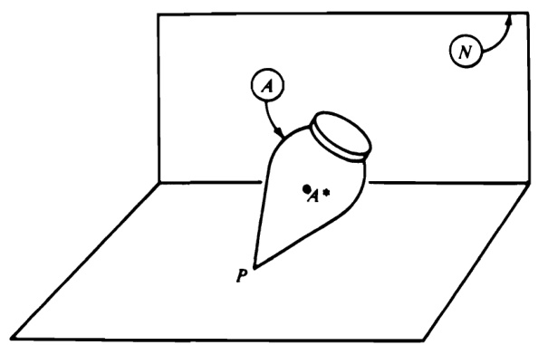
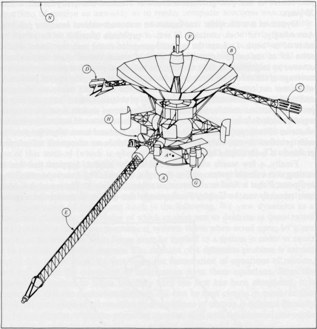
Finally, a few words about notation will be helpful. Suppose that one is dealing with a simple system, such as the top \pmb{A} , shown in Fig. i, the top terminating in a point P that is fixed in a Newtonian reference frame N . The notation needed here certainly can be simple. For instance, one can let \mathbf{\delta}\mathbf{o} denote the angular velocity of A in {\tilde{N}} andlet \mathbf{v} stand forthevelocityin N ofpoint A^{*} ,themass center of A Indeed,notations more elaborate than these can be regarded as objectionable because they burden the analyst with unnecessary writing.But suppose that one must undertake the analysis of motions of a complex system, such as the Galileo spacecraft,modeled as consisting of eight rigid bodies A,B,..., \# coupled to each other as indicated in Fig.ii.Here,unless one employsnotationsmore elaborate than \mathbf{\omega} and \mathbf{v} one cannot distinguish from each other such quantities as,say,the angular velocity of A in a Newtonian reference frame N the angular velocity of \boldsymbol{B} in N and the angular velocity of B in A ,all of which may enter the analysis. Or,if A^{*} and B^{*} arepoints ofinterest fixed on A and \boldsymbol{B} perhaps the respective mass centers, one needs a notation that permits one to distinguish from each other,say,the velocity of A^{*} in N the velocityof B^{*} in N andthevelocityof B^{*} in A Therefore,weestablish,and use consistently throughout this book, a few notational practices that work well in such situations. In particular, when a vector denoting an angular velocity or an angular acceleration of a rigid body in a certain reference frame has two superscripts, the right superscript stands for the rigid body, whereas the left superscript refers to the reference frame. Incidentally, we use the terms “reference frame' and “ rigid body " interchangeably. That is, every rigid body can serve as a reference frame, and every reference frame can be regarded as a massless rigid body. Thus, for example, the three angular velocities mentioned in connection with the system depicted in Fig. ii, namely, the angular velocity of \pmb{A} in N ,the angular velocity of \pmb{B} in N_{v} and the angular velocity of \pmb{B} in \pmb{A} , are denoted by \pmb{N}_{\mathbf{\mathbf{G}}\mathbf{\mathbf{D}}}\pmb{A} \mathbf{\bar{\mathit{N}}_{C D}}\mathbf{\mathit{B}} and \pmb{A_{\mathbb{Q}\tilde{\mathbf{D}}}}^{B} , respectively. Similarly, the right superscript on a vector denoting a velocity or acceleration of a point in a reference frame is the name of the point, whereas the left superscript identifies the reference frame. Thus, for example, the aforementioned velocity of A^{*} in N is written \aleph_{\mathbf{v}}A^{\star} and \pmb{A}_{\mathbf{V}}\pmb{B}^{*} represents the velocity of \pmb{{\cal B}}^{\ast} in \pmb{A} . Similar conventions are established in connection with angular momenta, kinetic energies, and so forth.

While there are distinct differences between our approach to dynamics, on the one hand, and traditional approaches, on the other hand, there is no fundamental conflict between the new and the old. On the contrary, the material in this book is entirely compatible with the classical literature. Thus, it is the purpose of this book not only to equip students with the skills they need to deal effectively with present-day dynamics problems, but also to bring them into position to interact smoothly with those trained more conventionally.

Thomas R. Kane David A. Levinson

Each of the seven chapters of this book is divided into sections. A section is identified by two numbers separated by a decimal point, the first number referring to the chapter in which the section appears, and the second identifying the section within the chapter. Thus, the identifier 2.14 refers to the fourteenth section of the second chapter. A section identifier appears at the top of each page.

Equations are numbered serially within sections. For example, the equations in Secs. 2.14 and 2.15 are numbered (1)-(31) and (1)-(50), respectively. References to an equation may be made both within the section in which the equation appears and in other sections. In the first case, the equation number is cited as a single number; in the second case, the section number is included as part of a threenumber designation. Thus, within Sec. 2.14, Eq. (2) of Sec. 2.14 is referred to as Eq. (2); in Sec. 2.15, the same equation is referred to as Eq. (2.14.2). To locate an equation cited in this manner, one may make use of the section identifiers appearing at the tops of pages.

Figures appearing in the chapters are numbered so as to identify the sections in which the figures appear. For example,the two figures in Sec. 4.8 are designated Fig. 4.8.1 and Fig. 4.8.2. To avoid confusing these figures with those in the problem sets and in Appendix I, the figure number is preceded by the letter \mathbf{P} in the case of problem set figures, and by the letter A in the case of Appendix I figures. The double number following the letter P refers to the problem statement in which the figure is introduced. For example, Fig. P12.3 is introduced in Problem 12.3. Similarly, Table 3.4.1 is the designation for a table in Sec. 3.4, and Table P14.6.2 is associated with Problem 14.6.

DIFFERENTIATION OF VECTORS

The discipline of dynamics deals with changes of various kinds, such as changes in the position of a particle in a reference frame, changes in the configuration of a mechanical system, and so forth. To characterize the manner in which some of these changes take place, one employs the differential calculus of vectors, a subject that can be regarded as an extension of material usually taught under the heading of the differential calculus of scalar functions. The extension consists primarily of provisions made to accommodate the fact that reference frames play a central role in connection with many of the vectors of interest in dynamics. For example, let \pmb{A} and \pmb{B} be reference frames moving relative to each other, but having one point o in common at all times, and let \pmb{P} be a point fixed in \pmb{A} , and thus moving in B. Then the velocity of \pmb{P} in \pmb{A} is equal to zero, whereas the velocity of \pmb{P} in \pmb{B} differs from zero. Now, each of these velocities is a time-derivative of the same vector, {\mathfrak{r}}^{o r}. the position vector from ^o to \pmb{P}_{\cdot} Hence, it is meaningless to speak simply of the time-derivative of {\mathsf{r}}^{o P} . Clearly, therefore, the calculus used to differentiate vectors must permit one to distinguish between differentiation with respect to a scalar variable in a reference frame \pmb{A} and differentiation with respect to the same variable in a reference frame \pmb{B}.

When working with elementary principles of dynamics, such as Newton's second law or the angular momentum principle, one needs only the ordinary differential calculus of vectors, that is, a theory involving differentiations of vectors with respect to a single scalar variable, generally the time. Consideration of advanced principles of dynamics, such as those presented in later chapters of this book, necessitates, in addition, partial differentiation of vectors with respect to several scalar variables, such as generalized coordinates and generalized speeds. Accordingly, the present chapter is devoted to the exposition of definitions, and consequences of these definitions, needed in the chapters that follow.

1.1 VECTOR FUNCTIONS

When either the magnitude of a vector \mathbf{v} and/or the direction of v in a reference frame A depends on a scalar variable q,\mathbf{v} is called a vector function of q in A. Otherwise, \mathbf{v} is said to be independent of \pmb q in \pmb{A}

Example In Fig. 1.1.1, \pmb{P} represents a point moving on the surface of a rigid sphere S, which, like any rigid body, may be regarded as a reference frame. (Reference frames should not be confused with coordinate systems. Many coordinate systems can be embedded in a given reference frame.) If \pmb{\Psi} is the position vector from the center c of s to point \pmb{P} , and if \pmb q_{1} and \pmb q_{2} are the angles shown, then \pmb{\mathbf{p}} is a vector function of \pmb q_{1} and \pmb q_{2} in \pmb{s} because the direction of \pmb{\mathbb{p}} in \boldsymbol{s} depends on \pmb q_{1} and q_{2} , but \pmb{\mathsf{p}} is independent of \pmb q_{3} in S, where \pmb q_{3} is the distance from c to a point \pmb R situated as shown in Fig. 1.1.1. The position vector r from c to \pmb R is a vector function of \pmb q_{3} in \pmb{S}, but is independent of \pmb q_{1} and \pmb q_{2} in S, and the position vector \pmb q from \pmb{P} to \pmb R is a vector function of \pmb q_{1} \boldsymbol{q}_{2} , and \pmb q_{3} in \pmb{S}

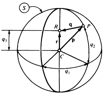
Figure 1.1.1

1.2 SEVERAL REFERENCE FRAMES

A vector v may be a function of a variable \pmb q in one reference frame, but be independent of \pmb q in another reference frame.

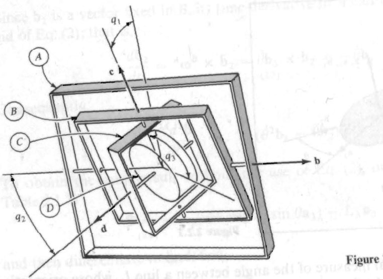
Example The outer gimbal ring \pmb{A} , inner gimbal ring \pmb{{\cal B}}, and rotor c of the gyroscope depicted in Fig. 1.2.1 each can be regarded as a reference frame. If p is the position vector from point ^o to a point \pmb{P} of c then p is a function of

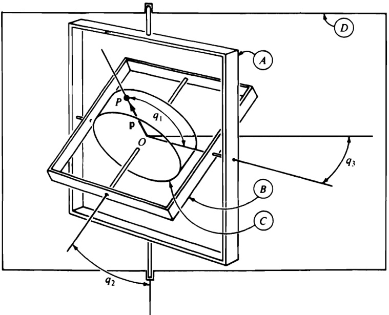
Figure 1.2.1

\pmb q_{1} both in \pmb{A} and in \pmb{B} but is independent of \pmb q_{1} in C;{p} is a function of \pmb{q_{2}} in \pmb{A} , but is independent of \pmb{q}_{2} both in \pmb{B} and in c ; and \pmb{P} is independent of \pmb q_{3} in each of A,B, and C , but is a function of \pmb q_{3} in reference frame \pmb{D}

1.3 SCALAR FUNCTIONS

Given a reference frame A and a vector function v of n scalar variables qi, ... , 9n in \pmb{A} let {\bf a}_{1},{\bf a}_{2},{\bf a}_{3} be a set of nonparallel, noncoplanar (but not necessarily mutually perpendicular) unit vectors fixed in \pmb{A} . Then there exist three unique scalar functions \pmb{v}_{1},\pmb{v}_{2},\pmb{v}_{3} of q_{1},\ldots,q_{n} such that

\mathbf{v}=v_{1}\mathbf{a}_{1}+v_{2}\mathbf{a}_{2}+v_{3}\mathbf{a}_{3}

This equation may be regarded as a bridge connecting scalar to vector analysis; it provides a convenient means for extending to vector analysis various important concepts familiar from scalar analysis, such as continuity, differentiability, and so forth. The vector \pmb{v}_{i}\pmb{\Omega}_{i} is called the {\bf{a}}_{i} component of \mathbf{v}. and \pmb{v_{i}} is known as the \mathbf{a}_{i} measure number of v (i = 1, 2, 3).

When \mathbf{a}_{1},\,\mathbf{a}_{2} ,and {\mathfrak{a}}_{3} are mutually perpendicular unit vectors, then it follows from Eq. (1) that the a; measure number of v is given by

v\!\!\!\!\!\!\!\!\!\!\!\!_{i}\!\!\!\!\!\!\!\!\!\!\!\!=\!\!\!\!\!\!\!\!\!\!\!\!1\!\!\!\!\!\!\!\!\!\!\!\!,\!\!\!\!\!\!\!\!\!\!\!\!\!\!\!\!\!\!\!\!\!\!\!(i\!\!\!\!\!\!\!\!\!\!\!\!\!\!)\!\!\!\!\!\!\!\!\!\!\!\!\!\!\!\!\!\!\!\!\!\!\!\!\!\!\!\!\!\!\!\!\!\!\!\!\!\!\!\!\!\!\!\!\!\!\!\!\!\!\!\!\!\!\!\!\!\!\!\!\!\!\!\!\!\!\!\!\!\!\!\!\!\!\!\!\!\!\!\!\!\!\!\!\!\!\!\!\!\!\!\!\!\!\!\!\!\!\!\!\!\!\!\!\!\!\!\!\!\!\!\!\!\!\!\!\!\!\!\!\!\!\!\!\!\!\!\!\!\!\!\!\!\!\!\!\!\!\!\!\!\!\!\!\!\!\!\!\!\!\!\!\!\!\!\!\!\!\!\!\!\!\!\!\!\!\!\!\!\!\!\!\!\!\!\!\!\!\!\!\!\!\!\!\!\!\!\!\!\!\!\!\!\!\!\!\!\!\!\!\!\!\!\!\!\!\!\!\!\!\!\!\!\!\!\!\!\!\!\!\!\!\!\!\!\!\!\!\!\!\!\!\!\!\!\!\!\!\!\!\!\!\!\!\!\!\!\!\!\!\!\!\!\!\!\!\!\!\!\!\!\!\!\!\!\!\!\!\!\!\!\!\!\!\!\!\!\!\!\!\!\!\!\!\!\!\!\!\!\!\!\!\!\!\!\!\!\!\!\!\!\!\!\!\!\!\!\!\!\!\!\!\!\!\!\!\!\!\!\!\!\!\!\!\!\!\!\!\!\!\!\!\!\!\!\!\!\!\!\!\!\!\!\!\!\!\!\!\!\!\!\!\!\!\!\!\!\!\!\!\!\!\!\!\!\!\!\!\!\!\!\!\!\!\!\!\!\!\!\!\!\!\!\!\!\!\!\!\!\!\!\!\!\!\!\!\!\!\!\!\!\!\!\!\!\!\!\!\!\!\!\!\!\!\!\!\!\!\!\!

and that Eq. (1) may, therefore, be rewritten as

{\bf v}={\bf v}\cdot{\bf a}_{1}{\bf a}_{1}+{\bf v}\cdot{\bf a}_{2}\,{\bf a}_{2}+{\bf v}\cdot{\bf a}_{3}\,{\bf a}_{3}

Conversely,if {\bf a}_{1},{\bf a}_{2} ,and {\bf a}_{3} are mutually perpendicular unit vectors and Eqs. (2) are regarded as definitions of v; (i = 1, 2, 3), then it follows from Eq. (3) that v can be expressed as in Eq. (1).

Example In Fig. 1.3.1, which shows the gyroscope considered in the example in Sec. 1.2, {\bf a}_{1} ， {\mathfrak{a}}_{2} ， {\bf a}_{3} and \mathbf{b}_{1},\,\mathbf{b}_{2},\,\mathbf{b}_{3} designate mutually perpendicular unit vectors fixed in \pmb{A} and in \pmb{B} , respectively. The vector p can be expressed both as

{\bf p}=\alpha_{1}{\bf a}_{1}+\alpha_{2}\,{\bf a}_{2}+\alpha_{3}\,{\bf a}_{3}

and as

\mathbf{p}=\beta_{1}\mathbf{b}_{1}+\beta_{2}\mathbf{b}_{2}+\beta_{3}\mathbf{b}_{3}

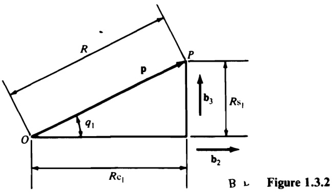
where \alpha_{i} and \beta_{i}\,(i=1,2,3) are functions of q_{1},q_{2} , and \boldsymbol{q}_{3} .To determine these functions, note that, if ^{c} has a radius \pmb R ,onecanproceedfrom o to P by moving through the distances \pmb R cOS q_{1} and \pmb R sin \pmb q_{1} in the directions of {\mathfrak{b}}_{2} and {\mathfrak{b}}_{3} (see Fig. 1.3.2), respectively, which means that

\mathbf{p}=R(\mathbf{c}_{1}\mathbf{b}_{2}+\mathbf{\beta}\mathbf{s}_{1}\mathbf{b}_{3})

where \mathbf{c}_{1} and \mathbf{s}_{1} are abbreviations for cos \pmb q_{1} and sin \pmb q_{1} , respectively. Comparing Eqs. (5) and (6), one thus finds that

\beta_{1}=0\qquad\beta_{2}=R\mathsf{c}_{1}\qquad\beta_{3}=R\mathsf{s}_{1}

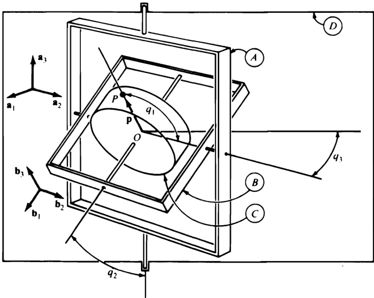
Figure 1.3.1

Moreover, in view of Eq. (4), one can writet

\begin{array}{r}{\mathfrak{x}_{1}=\mathfrak{p}\cdot\mathfrak{a}_{1}=R(\mathfrak{c}_{1}\mathfrak{b}_{2}\cdot\mathfrak{a}_{1}+\mathfrak{s}_{1}\mathfrak{b}_{3}\cdot\mathfrak{a}_{1})}\\ {\mathfrak{a}_{2}=\mathfrak{p}\cdot\mathfrak{a}_{2}=R(\mathfrak{c}_{1}\mathfrak{b}_{2}\cdot\mathfrak{a}_{2}+\mathfrak{s}_{1}\mathfrak{b}_{3}\cdot\mathfrak{a}_{2})}\\ {\mathfrak{a}_{3}=\mathfrak{p}\cdot\mathfrak{a}_{3}=R(\mathfrak{c}_{1}\mathfrak{b}_{2}\cdot\mathfrak{a}_{3}+\mathfrak{s}_{1}\mathfrak{b}_{3}\cdot\mathfrak{a}_{3})}\end{array}

From Fig. 1.3.1,

\begin{array}{r l}{\mathbf{b}_{2}\cdot\mathbf{a}_{1}=~0\qquad\mathbf{b}_{2}\cdot\mathbf{a}_{2}=1\qquad\mathbf{b}_{2}\cdot\mathbf{a}_{3}=~0}\\ {\mathbf{b}_{3}\cdot\mathbf{a}_{1}=\mathbf{c}_{2}\qquad\mathbf{b}_{3}\cdot\mathbf{a}_{2}=0\qquad\mathbf{b}_{3}\cdot\mathbf{a}_{3}=\mathbf{s}_{2}}\end{array}

Hence, the {\bf a}_{1},{\bf a}_{2},{\bf a}_{3} measure numbers of \pmb{\mathbb{p}} are

\alpha_{1}=R s_{1}c_{2}\qquad\alpha_{2}=\ R c_{1}\qquad\alpha_{3}\,=\,R s_{1}s_{2}

respectively.

1.4 FIRST DERIVATIVES

\mathbf{v} is a vector function of \pmb{n} scalar variables q_{1},\ldots,q_{n} in a reference frame A (see Sec. 1.1), then \pmb{n} vectors, called first partial derivatives of \mathbf{v} in \pmb{A} and denoted by the symbols

\frac{^{A}\!\partial\mathbf{v}}{\partial q_{r}}\quad\mathrm{or}\quad\frac{^{A}\!\partial}{\partial q_{r}}\left(\mathbf{v}\right)\quad\mathrm{or}\quad^{A}\!\partial\mathbf{v}/\partial q_{r}\qquad(r=1,\,\cdot\,\cdot\,,n)

^\dagger Numbers beneath signs of equality or beneath other symbols refer to equations numbered correspondingly.

are defined as follows: Let {\bf a}_{1},{\bf a}_{2},{\bf a}_{3} be any nonparallel, noncoplanar unit vectors fixed in \pmb{A} , and let \pmb{v}_{i} be the {\bf{a}}_{i} measure number of \mathbf{y} (see Sec. 1.3). Then

{\frac{A_{\partial\mathbf{v}}}{\partial q_{r}}}\triangleq\sum_{i=1}^{3}{\frac{\partial v_{i}}{\partial q_{r}}}\mathbf{a}_{i}\qquad(r=1,\ldots,n)

When \mathbf{v} is regarded as a vector function of only a single scalar variable in \pmb{A} -for instance the time t —then this definition reduces to that of the ordinary derivative of v with respect to t in \pmb{A} , that is, tot

{\frac{A}{d t}}\triangleq\sum_{i=1}^{3}{\frac{d v_{i}}{d t}}\,\mathbf{a}_{i}

Example The vector \pmb{\mathbf{p}} considered in the example in Sec. 1.3 possesses partial derivatives with respect to q_{1},\ q_{2} , and q_{3} in each of the reference frames A,\;B, and c . To form ^{4}\partial{\bf p}/\partial{\bf q}_{r} (r=1,2,3) , one can use the {\mathbf{a}}_{i} (i=1,2,3) measure numbers of \pmb{\mathsf{p}} available in Eqs. (1.3.13) and thus write

\frac{^{A}\!\partial\mathbf{p}}{\partial q_{r}}=\left[\frac{\partial}{\partial q_{r}}(R\mathrm{s}_{1}\mathrm{c}_{2})\right]\!\mathbf{a}_{1}\,+\,\left[\frac{\partial}{\partial q_{r}}(R\mathrm{c}_{1})\right]\mathbf{a}_{2}\,+\,\left[\frac{\partial}{\partial q_{r}}(R\mathrm{s}_{1}\mathrm{s}_{2})\right]\mathbf{a}_{3}\qquad(r=1,2,3)\,+\,h.c.,

Consequently,

\begin{array}{l}{{\displaystyle{\frac{A{\hat{\bf{0p}}}}{\partial q_{1}\mathbf{\Gamma}_{(3)}}}=R(\mathbf{c}_{1}\mathbf{c}_{2}\mathbf{a}_{1}-\mathbf{s}_{1}\mathbf{a}_{2}+\mathbf{c}_{1}\mathbf{s}_{2}\mathbf{a}_{3})}}\\ {~~}\\ {{\displaystyle{\frac{A{\hat{\bf{0p}}}}{\partial q_{2}\mathbf{\Gamma}_{(3)}}}=R\mathbf{s}_{1}(-\mathbf{s}_{2}\mathbf{a}_{1}+\mathbf{c}_{2}\mathbf{a}_{3})}}\\ {~~}\\ {{\displaystyle{\frac{A{\hat{\bf{0p}}}}{\partial q_{3}\mathbf{\Gamma}_{(3)}}}=0}}\end{array}

The last result agrees with the statement in the example in Sec. 1.2 that \pmb{\mathsf{p}} is independent of \boldsymbol{q}_{3} in \pmb{A}

Proceeding similarly to determine \displaystyle{^B\partial\mathbf{p}}/{\partial q_{r}}\,(r=1,2,3) , one obtains with the aid of Eqs. (1.3.7),

{\frac{^{B}\!\partial\mathbf{p}}{\partial q_{1}}}=R(-\,\mathbf{s}_{1}\mathbf{b}_{2}\,+\,\mathbf{c}_{1}\mathbf{b}_{3})\qquad{\frac{^{B}\!\partial\mathbf{p}}{\partial q_{2}}}=0\qquad{\frac{^{B}\!\partial\mathbf{p}}{\partial q_{3}}}=0

Finally, since \pmb{\Psi} is independent of q. (r=1,2,3) in c

\frac{c_{\hat{\partial}\mathbf{p}}}{\partial q_{r}}=0\qquad(r=1,2,3)

^{\dagger} The importance of reference frames in connection with time-differentiation of vectors is obscured by defining the ordinary derivative of a vector \blacktriangledown with respect to time t as the limit of \Delta\mathbf{v}/\Delta t as \pmb{\Delta t} approaches zero,for this fails to bring any reference frame into evidence.

Suppose now that \pmb q_{1} and \boldsymbol{q}_{2} are specified as explicit functions of time \boldsymbol{t} namely,

q_{1}=t\qquad q_{2}=2t\qquad q_{3}=3t

Then \alpha_{i}\,(i=1,2,3) of Eq. (1.3.4) can be expressed as [see Eqs. (1.3.13)]

\begin{array}{r}{\alpha_{1}=R\sin t\cos2t\qquad\alpha_{2}=R\cos t\qquad\alpha_{3}=R\sin t\sin2t}\end{array}

and the ordinary derivative of \blacktriangledown with respect to t in \pmb{A} is seen to be given by

\begin{array}{l}{{\displaystyle{\frac{{}A_{}{\bf{\dot{0}}}}{d t}}=\frac{d\alpha_{1}}{d t}{\bf\dot{a}}_{1}+\frac{d\alpha_{2}}{d t}{\bf\dot{a}}_{2}+\frac{d\alpha_{3}}{d t}{\bf\dot{a}}_{3}}\ ~}\\ {{\displaystyle~~~~~=~{\cal R}[(\cos t\cos2t-2\sin t\sin2t){\bf a}_{1}-\sin t{\bf\dot{a}}_{2}}\ ~}\\ {{\displaystyle~~~~~~+(\cos t\sin2t+2\sin t\cos2t){\bf a}_{3}]}\ ~}\end{array}

while the ordinary derivative of \pmb{\Psi} with respect to \boldsymbol{t} in \pmb{B} is [see Eqs. (1.3.7)]

{\frac{^{B}\!d{\bf p}}{d t}}=R(-\,\sin t\,\,{\bf b}_{2}\,+\,\cos\,t\,\,{\bf b}_{3})

Finally,

\frac{c_{d\mathfrak{p}}}{d t}=0

because, when \pmb{\mathbb{p}} is expressed as

\mathbf{p}=\gamma_{1}\mathbf{c}_{1}\,+\,\gamma_{2}\mathbf{c}_{2}\,+\,\gamma_{3}\mathbf{c}_{3}

where \mathbf{c}_{1},\mathbf{c}_{2},\mathbf{c}_{3} are unit vectors fixed in c , then \gamma_{1},\gamma_{2},\gamma_{3} are necessarily constants, \pmb{\Psi} being fixed in c

1.5 REPRESENTATIONS OF DERIVATIVES

When a partial or ordinary derivative of a vector v in a reference frame \pmb{A} is formed by carrying out the operations indicated in Eqs. (1.4.1) and (1.4.2), the resulting expression involves the unit vectors {\mathfrak{a}}_{1},{\mathfrak{a}}_{2},{\mathfrak{a}}_{3} , that is, unit vectors fixed in A. By expressing each of these unit vectors in terms of unit vectors \ b_{1},\ b_{2},\ b_{3} fixed in a reference frame \pmb{{\cal B}}, . one arrives at a new representation of the derivative under consideration, namely, one involving {\mathfrak{b}}_{1} ,\pmb{\mathrm{b}}_{2},\pmb{\mathrm{b}}_{3} , but one is still dealing with derivatives of \mathbf{v} in \pmb{A} , not in \pmb{B} , unless these two derivatives happen to be equal to each other.

Example Referring to Eq. (1.4.4) and noting (see Fig. 1.3.1) that

\mathbf{a}_{1}=\mathbf{s}_{2}\,\mathbf{b}_{1}\,+\,\mathbf{c}_{2}\,\mathbf{b}_{3}\qquad\mathbf{a}_{2}=\mathbf{b}_{2}\qquad\mathbf{a}_{3}=\,-\,\mathbf{c}_{2}\,\mathbf{b}_{1}\,+\,\mathbf{s}_{2}\,\mathbf{b}_{3}

one can write

\begin{array}{l}{\displaystyle\frac{{}^{A}\partial{\bf p}}{\partial q_{1}}=R[c_{1}c_{2}(s_{2}{\bf b}_{1}+\,c_{2}{\bf b}_{3})-\,s_{1}{\bf b}_{2}+\,c_{1}s_{2}(-c_{2}{\bf b}_{1}+\,s_{2}{\bf b}_{3})]}\\ {\displaystyle\qquad=R(-\,s_{1}{\bf b}_{2}+\,c_{1}{\bf b}_{3})}\end{array}

The right-hand sides of this equation and of the first of Eqs. (1.4.7) are identical. Hence, it appears that we have produced \;^{B}\!{\hat{O}}\!\,/\!{\hat{o}}q_{1} by expressing \mathbf{\nabla}^{A}\partial\mathbf{p}/\partial q_{1} in terms of \mathbf{b}_{1},\,\mathbf{b}_{2},\,\mathbf{b}_{3} . It was possible to do this because ^{\pm}\hat{\sigma}{\bf p}/\hat{\sigma}q_{1} and \mathfrak{s}_{\partial\mathbf{p}/\partial{q_{1}}} happen to be equal to each other. To see that the same procedure does not lead to {\mathfrak{s}}_{{\hat{O}}{\mathfrak{p}}/\partial q_{2}} when one starts with A_{\widehat{O}\,{\bf p}/\widehat{O}q_{2}} , refer to Eq. (1.4.5) to write, with the aid of Eqs. (1),

\begin{array}{l}{{\displaystyle\frac{{}^{A}\partial{\bf p}}{\partial q_{2}}=R s_{1}[-s_{2}(s_{2}\,{\bf b}_{1}\,+\,c_{2}\,{\bf b}_{3})\,+\,c_{2}(-\,c_{2}\,{\bf b}_{1}\,+\,s_{2}\,{\bf b}_{3})]}\ ~}\\ {{\mathrm{~\boldmath~\mu~}=\,-\,R s_{1}{\bf b}_{1}}}\end{array}

and compare this with the second of Eqs. (1.4.7)

1.6 NOTATION FOR DERIVATIVES

In general, both partial and ordinary derivatives of a vector v in a reference frame A differ from corresponding derivatives in any other reference frame B. It follows thatnotations such as \partial\mathbf{v}/\partial q_{\star} or d\mathbf{v}/d t -that is, ones that involve no mention of any reference frame —- are meaningful only either when the context in which they appear clearly implies a particular reference frame or when it does not matter which reference frame is used. In the sequel, it is to be understood that, whenever no reference frame is mentioned explicitly, any reference frame may be used, but all partial or ordinary differentiations indicated in any one equation are meant to be performed in the same reference frame.

Example The equations

{\bf p}\cdot\frac{\partial{\bf p}}{\partial q_{r}}=0\qquad(r=1,2,3)

and

\mathbf{p}\cdot{\frac{d\mathbf{p}}{d t}}=0

are valid for the vector p and the quantities q_{1},q_{2},q_{3} introduced in the example in Sec. 1.2, regardless of the reference frame in which \pmb{\mathsf{p}} is differentiated.We shall shortly be in a position to prove this. To verify it for a few specific cases, refer to Eqs. (1.3.6) and (1.4.7), which yield

\mathbf{p}\cdot{\frac{\mathbf{\nabla}^{B}\partial\mathbf{p}}{\partial q_{1}}}=R^{2}(\mathbf{c}_{1}\mathbf{b}_{2}+\mathbf{\nabla}\mathbf{s}_{1}\mathbf{b}_{3})\cdot(-\mathbf{s}_{1}\mathbf{b}_{2}+\mathbf{\nabla}\mathbf{c}_{1}\mathbf{b}_{3})=0

or use Eqs. (1.3.4), (1.3.13), and (1.4.5) to write

\mathbf{p}\cdot{\frac{^{A}\!\partial\mathbf{p}}{\partial q_{2}}}=R^{2}s_{1}(s_{1}c_{2}\mathbf{a}_{1}+c_{1}\mathbf{a}_{2}+s_{1}s_{2}\mathbf{a}_{3})\cdot(-s_{2}\mathbf{a}_{1}+c_{2}\mathbf{a}_{3})=0

Finally, note that Eqs. (1.3.4), (1.4.10), (1.4.11), and (1.4.13) lead to

\mathbf{p}\cdot{\frac{\mathbf{\nabla}\mathbf{}^{A}\partial\mathbf{p}}{d t}}=\mathbf{p}\cdot{\frac{c_{d\mathbf{p}}}{d t}}=0

1.7 DIFFERENTIATION OF SUMS AND PRODUCTS

As an immediate consequence of the definition given in Eqs. (1.4.1), the following rules govern the differentiation of sums and products involving vector functions.

\mathbf{v}_{1},\ldots,\mathbf{v}_{N} are vector functions of the scalar variables q_{1},\ldots,q_{n} in some reference frame, then

{\frac{\partial}{\partial q_{r}}}\sum_{i=1}^{N}\,\mathbf{v}_{i}=\sum_{i=1}^{N}{\frac{\partial\mathbf{v}_{i}}{\partial q_{r}}}\qquad(r=1,\ldots,n)

\boldsymbol{s} is a scalar function of q_{1},\ldots,q_{n} , and \mathbf{v} and \mathbf{w} are vector functions of these variables in some reference frame, then

\begin{array}{c c}{\displaystyle\frac{\partial}{\partial q_{r}}(s\mathbf{v})=\frac{\partial s}{\partial q_{r}}\mathbf{v}+s\frac{\partial\mathbf{v}}{\partial q_{r}}}&{(r=1,\ldots,n)}\\ {\displaystyle\frac{\partial}{\partial q_{r}}(\mathbf{v}\cdot\mathbf{w})=\frac{\partial\mathbf{v}}{\partial q_{r}}\mathbf{\cdotw}+\mathbf{v}\cdot\frac{\partial\mathbf{w}}{\partial q_{r}}}&{(r=1,\ldots,n)}\\ {\displaystyle\frac{\partial}{\partial q_{r}}(\mathbf{v}\times\mathbf{w})=\frac{\partial\mathbf{v}}{\partial q_{r}}\times\mathbf{w}+\mathbf{v}\times\frac{\partial\mathbf{w}}{\partial q_{r}}}&{(r=1,\ldots,n)}\end{array}

More generally, if \pmb{P} is the product of N scalar and/or vector functions F_{i}\left(i=\right. 1,\ldots,N), that is, if

P=F_{1}F_{2}\cdots F_{N}

then,if al symbols of operation, such as dots, crosses, and parentheses, are kept in place,

\frac{\d^{1}P}{\d q_{r}}=\frac{\partial F_{1}}{\partial q_{r}}F_{2}\cdot\cdot\cdot F_{N}+F_{1}\frac{\partial F_{2}}{\partial q_{r}}\cdot\cdot\cdot F_{N}+\cdot\cdot\cdot+F_{1}F_{2}\cdot\cdot\cdot F_{N-1}\frac{\partial F_{N}}{\partial q_{r}}\quad(r=1,...+F_{N})\frac{\partial F_{N}}{\partial q_{r}}.

Relationships analogous to Eqs. (1)-(6) govern the ordinary diferentiation [see Eq. (1.4.2)] of vector and/or scalar functions of a single scalar variable.

Example By definition,the square of a vector \mathbf{v} ,written \mathbf{v}^{2} ,is the scalar quantity obtained by dot-multiplying \mathbf{v} with v. Hence, if \pmb{s} is a scalar function of q_{1},\ldots,q_{n} , then

{\begin{array}{r l}&{{\cfrac{\partial}{\partial q_{r}}}(s\mathbf{v}^{2})={\cfrac{\partial}{\partial q_{r}}}(s\mathbf{v}\cdot\mathbf{v})}\\ &{\qquad\qquad={\cfrac{\partial s}{\partial q_{r}}}\,\mathbf{v}\cdot\mathbf{v}+s\,{\cfrac{\partial\mathbf{v}}{\partial q_{r}}}\cdot\mathbf{v}+s\mathbf{v}\cdot{\cfrac{\partial\mathbf{v}}{\partial q_{r}}}\qquad(r=1,\ldots,n)}\end{array}}

or, since the last two terms are equal to each other,

{\frac{\partial}{\partial q_{r}}}(s\mathbf{v}^{2})={\frac{\partial s}{\partial q_{r}}}\,\mathbf{v}^{2}\,+\,2s\mathbf{v}\cdot{\frac{\partial\mathbf{v}}{\partial q_{r}}}\qquad(r=1,\ldots,n)

This result can be used to establish the validity of Eqs. (1.6.1) by taking s=1 ? Writing \pmb{\mathbb{P}} inplaceof \mathbf{v} andletting n=3 whichyields

{\frac{\partial}{\partial q_{r}}}({\bf p}^{2})=2{\bf p}\cdot{\frac{\partial{\bf p}}{\partial q_{r}}}\qquad(r=1,2,3)

and then noting that, for the vector \pmb{\mathsf{p}} in Eqs. (1.6.1), {\mathfrak{p}}^{2} is a constant, so that

\frac{\partial}{\partial q_{r}}({\bf p}^{2})=0\qquad(r=1,2,3)

Since \scriptstyle2\;\neq\;0 , Eqs. (9) and (10) imply that

{\bf p}\cdot\frac{\partial{\bf p}}{\partial q_{r}}=0\qquad(r=1,2,3)

in agreement with Eqs. (1.6.1)

1.8 SECOND DERIVATIVES

In general, \mathbf{\nabla}^{A}\partial\mathbf{v}/\partial q, (see Sec. 1.4) is a vector function of q_{1},\ldots,q_{n} both in \pmb{A} and in any other reference frame \pmb{B} and can, therefore, be differentiated with respect to any one of q_{1},\ldots,q_{n} both in \pmb{A} and in \pmb{B}. The result of such a differentiation is called a second partial derivative. Similarly, the ordinary derivative \mathbf{\nabla}^{A}d\mathbf{v}/d t (see Sec. 1.4) can be differentiated with respect to t both in \pmb{A} and in any other reference frame \pmb{B}

The order in which successive differentiations are performed can affect the results. For example, in general,

\frac{^{B}\!\partial}{\partial q_{s}}\left(\frac{^{A}\!\partial\mathbf{v}}{\partial q_{r}}\right)\neq\frac{^{A}\!\partial}{\partial q_{r}}\left(\frac{^{B}\!\partial\mathbf{v}}{\partial q_{s}}\right)\quad\mathrm{~}(r,s=1,\ldots,n)

and

\frac{b}{d t}\left(\frac{A_{d}\mathbf{v}}{d t}\right)\neq\frac{A}{d t}\left(\frac{B_{d}\mathbf{v}}{d t}\right)

However, if successive partial differentiations with respect to various variables are performed in the same reference frame, then the order is immaterial; that is,

{\frac{\partial}{\partial q_{s}}}\left({\frac{\partial\mathbf{v}}{\partial q_{r}}}\right)={\frac{\partial}{\partial q_{r}}}\left({\frac{\partial\mathbf{v}}{\partial q_{s}}}\right)\qquad(r,s=1,\ldots,n)

and

{\frac{\partial}{\partial t}}\left({\frac{\partial\mathbf{v}}{\partial q_{r}}}\right)={\frac{\partial}{\partial q_{r}}}\left({\frac{\partial\mathbf{v}}{\partial t}}\right)\qquad(r=1,\ldots,n)

Example Referring to the example in Sec. 1.3, suppose that a vector \mathbf{v} is given by

\mathbf{v}=t\mathbf{a}_{1}

and that q_{2} is a specified function of t, Then

\frac{{\mathbf{\nabla}}A\mathbf{v}}{d t}=\mathbf{a}_{1}\mathbf{\Phi}=\mathbf{\Phi}\mathbf{s}_{2}\mathbf{b}_{1}+\mathbf{c}_{2}\mathbf{b}_{3}

and

\frac{^{B}\!d}{d t}\left(\frac{^{A}\!d\mathbf{v}}{d t}\right)=\dot{q}_{2}(\mathbf{c}_{2}\mathbf{b}_{1}-\mathbf{s}_{2}\mathbf{b}_{3})\mathbf{\Omega}_{(1,5,1)}-\dot{q}_{2}\mathbf{a}_{3}

Also,

\mathbf{v}=t(s_{2}\,\mathbf{b}_{1}+c_{2}\,\mathbf{b}_{3})

so that

{\begin{array}{l l l}{{\cfrac{^{B}\!d\mathbf{v}}{d t}}}&{=}&{{\cfrac{d t}{d t}}\,(s_{2}\mathbf{b}_{1}+c_{2}\mathbf{b}_{3})+t\,{\cfrac{^{B}\!d}{d t}}\,(s_{2}\mathbf{b}_{1}+c_{2}\mathbf{b}_{3})}\\ &{}&\\ &{=}&{s_{2}\mathbf{b}_{1}+c_{2}\mathbf{b}_{3}+t{\dot{q}}_{2}(c_{2}\mathbf{b}_{1}-s_{2}\mathbf{b}_{3})}\\ &{}&\\ &{=}&{\mathbf{a}_{1}-t{\dot{q}}_{2}\mathbf{a}_{3}}\\ &{}&\end{array}}

and

\frac{A_{d}}{d t}\left(\frac{{\tt^{B}}d{\tt v}}{d t}\right)\,=\,-\,(\dot{q}_{2}\,+\,t\ddot{q}_{2}){\bf a}_{3}

Comparing Eqs. (7) and (10), one sees that, in general, one must expect the result of successive differentiations in various reference frames to depend on the order in which the differentiations are performed.

1.9 TOTAL AND PARTIAL DERIVATIVES

q_{1},\ldots,q_{n} are scalar functions of a single variable t it is sometimes convenient to regard a vector \mathbf{v} as a vector function of the n+1 independent variables q_{1},\ldots,q_{n} , and t in a reference frame \pmb{A} . The ordinary derivative of \mathbf{v} with respect to t in \pmb{A} (see Sec. 1.4), called a total derivative under these circumstances, then can be expressed in terms of partial derivatives as

\frac{A\times}{d t}=\sum\limits_{r=1}^{n}\frac{A_{0}\times}{\partial{q}_{r}}\dot{q}_{r}+\frac{A_{0}\times}{d t}=\frac{\dot{\zeta}\times\zeta}{c^{\prime}}\cdot\frac{\dot{\zeta}^{\prime}}{3!}+\dot{\zeta}^{\prime}\dot{\zeta}^{\prime}\dot{\zeta}^{\prime}(1)

where {\dot{q}}, . denotes the first derivative of \pmb q_{i} with respect to t . Moreover, if \mathbf{v} is differentiated both totally with respect to t and partially with respect to q_{r} , then the order in which the differentiations are performed is immaterial; that is,

{\frac{d}{d t}}{\frac{\partial\mathbf{v}}{\partial q_{r}}}={\frac{\partial}{\partial q_{r}}}{\frac{d\mathbf{v}}{d t}}\qquad(r=1,\ldots,n)

Derivations Let {\bf\&}_{i} (i=1,2,3) be nonparallel, noncoplanar unit vectors fixed in \pmb{A} , and regard \pmb{v}_{i} , the {\bf{a}}_{i} measurenumberof \mathbf{v} (see Sec. 1.3), as a function of q_{1},\ldots,q_{n} , and t From scalar calculus,

{\frac{d v_{i}}{d t}}=\sum_{r=1}^{n}\!{\frac{\partial v_{i}}{\partial q_{r}}}{\dot{q}}_{r}+{\frac{\partial v_{i}}{\partial t}}\qquad(i=1,2,3)

and, if m and q_{m} are defined as

m\triangleq n+1

and

\smash{q_{m}\triangleq t}

so that

\dot{q}_{m}=1

then Eqs. (3) can be rewritten as

{\frac{d v_{i}}{d t}}=\sum_{r=1}^{n}{\frac{\partial v_{i}}{\partial q_{r}}}{\dot{q}}_{r}+{\frac{\partial v_{i}}{\partial q_{m}}}{\dot{q}}_{m}=\sum_{r=1}^{m}{\frac{\partial v_{i}}{\partial q_{r}}}{\dot{q}}_{r}\ \ \ \ \ (i=1,2,3)

and substitution into Eq. (1.4.2) yields

\begin{array}{l}{{\displaystyle{\frac{{\cal A}}{d t}}\displaystyle=\sum_{i=1}^{3}\left(\sum_{r=1}^{m}\frac{\partial v_{i}}{\partial q_{r}}\dot{q}_{r}\right)\!\mathbf{a}_{i}=\sum_{r=1}^{m}\Bigg(\displaystyle\sum_{i=1}^{3}\frac{\partial v_{i}}{\partial q_{r}}\mathbf{a}_{i}\Bigg)\dot{q}_{r}}}\\ {{\displaystyle=\sum_{r=1}^{m}\;\frac{{\cal A}\partial{\bf v}}{\partial q_{r}}\;\dot{q}_{r}=\sum_{r=1}^{n}\frac{{\cal A}\partial{\bf v}}{\partial q_{r}}\;\dot{q}_{r}+\frac{{\cal A}\partial{\bf v}}{\partial q_{m}}\,\dot{q}_{m}}}\end{array}

which, in view of Eqs. (5) and (6), establishes the validity of Eq. (1). Furthermore, replacing \mathbf{v} in Eq. (1) with \partial\mathbf{v}/\partial q_{s} produces

\begin{array}{r l}{\displaystyle\frac{d}{d t}\frac{\partial\mathbf{v}}{\partial q_{s}}}&{={}\,\sum_{r=1}^{n}\left[\frac{\partial}{\partial q_{r}}\left(\frac{\partial\mathbf{v}}{\partial q_{s}}\right)\right]\dot{q}_{r}+\frac{\partial}{\partial t}\left(\frac{\partial\mathbf{v}}{\partial q_{s}}\right)}\\ {\displaystyle}&{={}\,\sum_{r=1}^{n}\left[\frac{\partial}{\partial q_{s}}\left(\frac{\partial\mathbf{v}}{\partial q_{r}}\right)\right]\dot{q}_{r}+\frac{\partial}{\partial q_{s}}\left(\frac{\partial\mathbf{v}}{\partial t}\right)}\\ {\displaystyle}&{={}\,\frac{\partial}{\partial q_{s}}\left(\sum_{r=1}^{n}\frac{\partial\mathbf{v}}{\partial q_{r}}\dot{q}_{r}+\frac{\partial\mathbf{v}}{\partial t}\right)}\\ {\displaystyle}&{={}\,\frac{\partial}{\partial q_{s}}\frac{d\mathbf{v}}{\partial q_{s}}\frac{\partial\mathbf{v}}{d t}\quad(s=1,\dots,n)}\end{array}

in agreement with Eq. (2).

Example To see that one can proceed in a variety of ways to find the ordinary derivative of a vector function in a reference frame, consider once more the vector \pmb{\Psi} introduced in the example in Sec. 1.3, and again let q_{1},q_{2} , and \boldsymbol{q}_{3} be given by Eqs. (1.4.9). Then the ordinary time-derivative of \pmb{\nu} in \pmb{A} previously found by using Eq. (1.4.2), is given by Eq. (1.4.11). Now refer to Eqs. (1.3.4) and (1.3.13) to express p as

\mathbf{p}=R(\mathtt{s}_{1}\mathtt{c}_{2}\,\mathbf{a}_{1}\,+\,\mathtt{c}_{1}\mathbf{a}_{2}\,+\,\mathtt{s}_{1}\mathtt{s}_{2}\,\mathbf{a}_{3})

and use Eqs. (1.4.9) to rewrite the {\mathfrak{a}}_{3} measure number of \pmb{\mathsf{p}} as an explicit function of t , that is, to replace Eq. (10) with

{\bf p}=R({\bf s}_{1}{\bf c}_{2}\,{\bf a}_{1}\,+\,{\bf c}_{1}{\bf a}_{2}\,+\,\sin\,t\,\sin\,2t\,{\bf a}_{3})

Furthermore, regard \pmb{\mathsf{p}} as a function of the independent variables q_{1},q_{2},q_{3} ， and t and then appeal to Eq. (1) to write

\begin{array}{c}{{{\displaystyle{\frac{{\bf{\cal A}}}{d t}}{\bf\tilde{\Delta}}={\frac{{\bf{\cal A}}}{\partial q_{1}}}{\dot{q}}_{1}\,+{\frac{{\bf{\cal A}}}{\partial q_{2}}}{\dot{q}}_{2}\,+{\frac{{\cal A}}{\partial q_{3}}}{\dot{q}}_{3}\,+{\frac{{\cal A}}{\partial t}}{\bf\tilde{\Delta}}}}\\ {{{\cal\qquad}=\,{\cal R}[({\bf c}_{1}{\bf c}_{2}{\bf a}_{1}\,-{\bf\,s}_{1}{\bf a}_{2}){\dot{q}}_{1}\,+(-{\bf\,s}_{1}{\bf s}_{2}{\bf a}_{1}){\dot{q}}_{2}}}\\ {{{\nonumber}}}\\ {{{\qquad+{\bf\,(c o s\,\,t i s i n\,2}t+2\,\sin{\bf\,}t\cos{2t}){\bf a}_{3}]}}}\end{array}

Finally, make the substitutions [see Eqs. (1.4.9)]

\begin{array}{r l r l}{\dot{q}_{1}=1}&{{}}&{s_{1}=\sin t}&{{}\quad\mathtt{c}_{1}=\cos t}\\ {\dot{q}_{2}=2}&{{}}&{s_{2}=\sin2t}&{{}\quad\mathtt{c}_{2}=\cos2t}\end{array}

and verify that the resulting equation is precisely Eq. (1.4.11). The point here is not that use of Eq. (1) facilitates the evaluation of ordinary derivatives; indeed, it may complicate matters. What is important is to realize that one may treat the same vector in a variety of ways, that the formalism one uses to construct the ordinary derivative of the vector in a given reference frame depends on the functional character one attributes to the vector, but that the result one obtains is independent of the approach taken. In the sequel, Eq. (1) will be used primarily in the course of certain derivations, rather than for the actual evaluation of ordinary derivatives.

Chapter 2 KINEMATICS

Considerations of kinematics play a central role in dynamics Indeed, one's efectiveness in formulating equations of motion depends primarily on one's ability to construct corrct mathematical expressions for kinematical quantities such as angular velocities of rigid bodies, velocities of points, and so forth. Therefore, mastery of the material in this chapter is essential.

The sections that follow can be divided into four groups. Sections 2.1-2.5, Which form the first group,are concerned with rotational motion of a rigid body. The principal kinematical quantity introduced here is the angular velocity of a rigid bodyin a refrence frame. Next, translational motion of a point is treated in Sec.26-2.8where four theorems frequentlyused in practice are derived from defnitions of the velocity and acceleration of a point in a reference frame. The reason for discussing translational motion after rotational motion is that the theorems on translational motion in Secs. 2.6-2.8 involve angular velocities and angular accelerations of rigid bodies, whereas the material on rotational motion inSec. 2.2does ot involve velocities oraccelrations of points.Thereaf, in Secs. 2.9-2.13,the subject of constraints is examined in detail,and mathematical techniques for dealing with constraints are presented in terms involving generalized coordinates and generalized speeds. Finally, partial angular velocities of a rigid body and partialvelcities ofa point areat thefocusofattentionnecs.2.14and 2.15. It is these quantities that ultimately enable one to form in a straightforward manner the terms that make up dynamical equations of motion.

2.1 ANGULAR VELOCITY

The use of angular velocities greatly facilitates the analysis of motions of systems containing rigid bodies. We begin our discussion of this topic with a formal definition of angular velocity; while it is abstract, this definition provides a sound basis for the derivation of theorems [see, for example, Eq. (2)] used to solve physical problems. ^{\dagger}

Let \ b_{1},\ b_{2} ， {\bf b}_{3} form a right-handed set of mutually perpendicular unit vectors fixed in a rigid body \pmb{B} moving in a reference frame \pmb{A} .The angular velocity of \pmb{B} in \pmb{A} , denoted by {\bf{ }}^{A}{\bf{\omega}}^{B} , is defined as

{\bf{ }}^{A}{\bf{\omega}}^{B}\triangleq{\bf{b}}_{1}\,\frac{{{\bf{ }}}^{A}d{\bf{b}}_{2}}{d t}\cdot{\bf{b}}_{3}\,+\,{\bf{b}}_{2}\,\frac{{{\bf{ }}}^{A}d{\bf{b}}_{3}}{d t}\,\cdot{\bf{b}}_{1}\,+\,{\bf{b}}_{3}\,\frac{{{\bf{ }}}^{A}d{\bf{b}}_{1}}{d t}\cdot{\bf{b}}_{2} \tag{1}

One task facilitated by the use of angular velocity vectors is the time-differentiation of vectors fixed in a rigid body, for it enables one to obtain the first timederivative of such a vector by performing a cross-multiplication. Specifically, if \beta is any vector fixed in \pmb{B}. then

{\frac{{\mathbf{ }}^{A}d{\beta}}{d t}}={\mathbf{}}^{A}\omega^{B}\times{{\beta}}\tag{2}

Derivation Using dots to denote time-differentiation in \pmb{A} , one can rewrite Eq. (1)as

{\bf{ }}^{A}{\bf{\omega}}^{B}\triangleq{\bf b}_{1}\dot{\bf b}_{2}\cdot{\bf b}_{3}+{\bf b}_{2}\dot{\bf b}_{3}\cdot{\bf b}_{1}+{\bf b}_{3}\dot{\bf b}_{1}\cdot{\bf b}_{2}\tag{3}

and cross-multiplication of Eq. (3) with {\bf b}_{1} gives

{\bf{ }}^{A}{\bf{\omega}}^{B}\times\,{\bf{b}}_{1}={\bf{b}}_{2}\times{\bf}{\bf{b}}_{1}{\bf{\dot{b}}}_{3}\cdot{\bf{b}}_{1}+{\bf{b}}_{3}\times{\bf}{\bf{b}}_{1}{\bf{\dot{b}}}_{1}\cdot{\bf{b}}_{2}\tag{4}

Now,since \mathbf{b}_{1},\,\mathbf{b}_{2},\,\mathbf{b}_{3} form a right-handed set of mutually perpendicular unit vectors, each can be expressed as a cross-product involving the remaining two. For example,

\mathbf{b}_{2}=\mathbf{b}_{3}\times\mathbf{b}_{1}\qquad\mathbf{b}_{3}=\mathbf{b}_{1}\times\mathbf{b}_{2}\tag{5}

and substitution into Eq. (4) yields

{\bf{ }}^{A}{\bf{\omega}}^{B}\times\mathbf{b}_{1}=-{\bf b}_{3}\,{\bf\dot{b}}_{3}\cdot{\bf b}_{1}+{\bf b}_{2}\,{\bf\dot{b}}_{1}\cdot{\bf b}_{2}\tag{6}

Moreover, time-differentiation of the equations {{b}}_{1}\cdot{{b}}_{1}=1 and {\bf b}_{3}\cdot{\bf b}_{1}=0 produces

\mathbf{\dot{b}}_{1}\cdot\mathbf{b}_{1}=0\qquad\mathbf{\dot{b}}_{3}\cdot\mathbf{b}_{1}=\mathbf{}-\mathbf{\dot{b}}_{1}\cdot\mathbf{b}_{3}\tag{7}

and with the aid of these one can rewrite Eq. (6) as

{\bf{ }}^{A}{\bf{\omega}}^{B}\times{\bf\dot{b}}_{1}={\bf b}_{1}{\bf\dot{b}}_{1}\cdot{\bf b}_{1}+{\bf b}_{2}{\bf\dot{b}}_{1}\cdot{\bf b}_{2}+{\bf b}_{3}{\bf\dot{b}}_{1}\cdot{\bf b}_{3}\tag{8}

^\dagger The frequently employed definition of angular velocity as the limit of \Delta\pmb{\theta}/\Delta t as \pmb{\Delta t} approaches zero is deficient in this regard.

But the right-hand member of this equation is simply a way of writing {\dot{\mathbf{b}}}_{1} [see Eq. (1.3.3)]. Consequently,

{}^{A}{\omega}^{B}\times{\bf b}_{1}={\bf\dot{b}}_{1}\tag{9}

Similarly,

{}^{A}{\omega}^{B}\times{\bf\dot{b}}_{2}={\bf\dot{b}}_{2}, \qquad{}^{A}{\omega}^{B}\times{\bf\dot{b}}_{3}={\bf\dot{b}}_{3}\tag{10}

and, after expressing any vector \upbeta fixed in \pmb{B} as

\beta=\beta_{1}\mathbf{b}_{1}+\beta_{2}\mathbf{b}_{2}+\beta_{3}\mathbf{b}_{3}\tag{11}

where \beta_{1},\,\beta_{2},\,\beta_{3} are constants, so that

\dot{\pmb{\beta}}\,=\,\beta_{1}\dot{\bf b}_{1}+\beta_{2}\dot{\bf b}_{2}+\beta_{3}\dot{\bf b}_{3}\tag{12}

one arrives at

\begin{array}{r l r}&{}&{\dot{\beta}\;=\;\beta_{1}{}^{A}\mathfrak{\omega}^{B}\times\,b_{1}+\beta_{2}{}^{A}\mathfrak{\omega}^{B}\times\,b_{2}+\beta_{3}{}^{A}\mathfrak{\omega}^{B}\times\,b_{3}}\\ &{}&{(10)\qquad\qquad\qquad\qquad\qquad\qquad\qquad(10)}\\ &{}&{=\;{}^{A}\mathfrak{\omega}^{B}\times(\beta_{1}{b}_{1}+\beta_{2}{b}_{2}+\beta_{3}{b}_{3})\;=\;{}^{A}\mathfrak{\omega}^{B}\times\,{b}}\end{array}

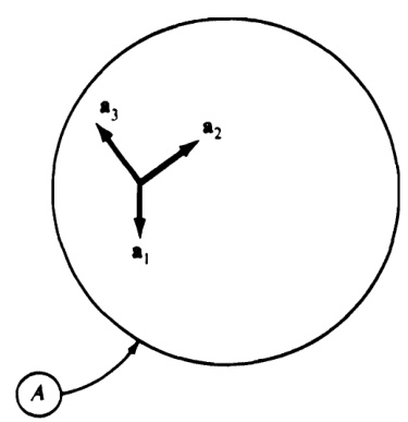
Examples Figure 2.1.1 shows a rigid satellite \pmb{B} in orbit about the Earth \pmb{A} A dextral set of mutually perpendicular unit vectors \mathbf{b}_{1},\,\mathbf{b}_{2},\,\mathbf{b}_{3} is fixed in \pmb{B} and a similar such set, {{a}}_{1},\,{{a}}_{2},\,{{a}}_{3} , is fixed in \pmb{A} Measurements are made to determine the time-histories of \alpha_{i},\beta_{i},\gamma_{i} , defined as

\alpha_{i}\triangleq\mathbf{b}_{1}\cdot\mathbf{a}_{i}\qquad\beta_{i}\triangleq\mathbf{b}_{2}\cdot\mathbf{a}_{i}\qquad\gamma_{i}\triangleq\mathbf{b}_{3}\cdot\mathbf{a}_{i}\qquad(i=1,2,3)

as well as the time-histories of \dot{\alpha}_{i},\,\dot{\beta}_{i},\,\dot{\gamma}_{i} , defined as the time-derivatives of \alpha_{i},\,\beta_{i},\,\gamma_{i} , respectively. At a certain time t^{*} , these quantities have the values

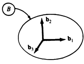
Figure 2.1.1

recorded in Tables 2.1.1 and 2.1.2. The angular velocity of \pmb{B} in \pmb{A} at time t^{*} is to be determined.

Table 2.1.1

<html>

1	α;	β:	Yi
1	0.9363	-0.2896	0.1987
2	0.3130	0.9447	-0.0981
3	-0.1593	0.1540	0.9751

</html>

Table 2.1.2

<html>

	αi (rad/s)	β; (rad/s)	(rad/s)
1 2 3	-0.0127 0.0303 -0.0148	-0.0261 -0.0103 0.0145	0.0216 -0.0032 -0.0047

</html>

It follows from Eqs. (14) that

\begin{array}{r}{\mathbf{b}_{1}=\alpha_{1}\mathbf{a}_{1}+\alpha_{2}\mathbf{a}_{2}+\alpha_{3}\mathbf{a}_{3}}\\ {\mathbf{b}_{2}=\beta_{1}\mathbf{a}_{1}+\beta_{2}\mathbf{a}_{2}+\beta_{3}\mathbf{a}_{3}}\end{array}

and

\mathbf{b}_{3}=\gamma_{1}\mathbf{a}_{1}+\gamma_{2}\mathbf{a}_{2}+\gamma_{3}\mathbf{a}_{3}

Consequently, for all values of the time t

\begin{array}{l}{{\displaystyle\frac{{\displaystyle}A{\bf j}_{1}}{{\displaystyle d t}_{\mathrm{~(15)}}}}={\dot{\alpha}}_{1}{\bf a}_{1}+{\dot{\alpha}}_{2}{\bf a}_{2}+{\dot{\alpha}}_{3}{\bf a}_{3}}\\ {~~}\\ {{\displaystyle\frac{{\displaystyle}A{\bf j}_{2}}{{\displaystyle d t}_{\mathrm{~(16)}}}}={\dot{\beta}}_{1}{\bf a}_{1}+{\dot{\beta}}_{2}{\bf a}_{2}+{\dot{\beta}}_{3}{\bf a}_{3}}\\ {~~}\\ {{\displaystyle\frac{{\displaystyle}A{\bf j}_{3}}{{\displaystyle d t}_{\mathrm{~(17)}}}}={\dot{\gamma}}_{1}{\bf a}_{1}+{\dot{\gamma}}_{2}{\bf a}_{2}+{\dot{\gamma}}_{3}{\bf a}_{3}}\end{array}

and

\begin{array}{c}{{{\cal A}_{\bf0}{}^{B}={\bf b}_{1}(\dot{\beta}_{1}\gamma_{1}+\dot{\beta}_{2}\gamma_{2}+\dot{\beta}_{3}\gamma_{3})+{\bf b}_{2}(\dot{\gamma}_{1}\alpha_{1}+\dot{\gamma}_{2}\alpha_{2}+\dot{\gamma}_{3}\alpha_{3})}}\\ {{{\mathrm{\boldmath~\Lambda~}}^{(1)}\qquad\qquad\qquad(19.17)}}\\ {{+{\bf\delta b}_{3}(\dot{\alpha}_{1}\beta_{1}+\dot{\alpha}_{2}\beta_{2}+\dot{\alpha}_{3}\beta_{3})}}\\ {{{\mathrm{\boldmath~\Lambda~}}^{(18,16)}}}\end{array}

Thus, at time t^{*} , Eq. (21) together with Tables 2.1.1 and 2.1.2 yields

{\pmb{\omega}}^{B}=0.010{\pmb{\ b}}_{1}+0.020{\pmb{\ b}}_{2}+0.030{\pmb{\ b}}_{3}\qquad\mathrm{rad/s}

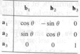
In Fig. 2.1.2, \pmb{B} represents a door supported by hinges in a room \pmb{A} Mutually perpendicular unit vectors {\mathfrak{a}}_{1},{\mathfrak{a}}_{2},{\mathfrak{a}}_{3} are fixed in \pmb{A} with {\mathfrak{a}}_{3} parallel to the axis of the hinges, and mutually perpendicular unit vectors \mathbf{b}_{1},\mathbf{b}_{2},\mathbf{b}_{3} are fixed in \pmb{B}, with {\mathfrak{b}}_{3}={\mathfrak{a}}_{3} . If \theta is the radian measure of the angle between {\mathfrak{a}}_{1} and {\bf b}_{1} , as shown in Fig. 2.1.2, then {\mathfrak{a}}_{1},{\mathfrak{a}}_{2},{\mathfrak{a}}_{3} and \mathbf{b}_{1},\mathbf{b}_{2},\mathbf{b}_{3} are related to each other as indicated in Table 2.1.3.

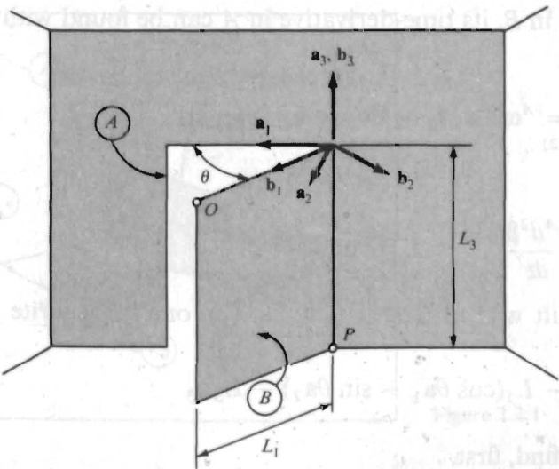
Figure 2.1.2

Table 2.1.3

The angular velocity of B A,\,{^{A}{\bf\L_{O}}^{B}}, foundwith the aidofEq.(1）andTable 2.1.3, is given byt

{}^{A}\mathbf{\epsilon}\mathbf{o}^{B}=\dot{\theta}\mathbf{b}_{3}

and theutility ofEq.(2)becomes apparentwhenone seekstofind,orxample,the second time-derivative in A of the position vector from the point Oshown inFig.2.1.2to the pointP,that isof the vectorβ given by

\beta=-L_{1}\mathbf{b}_{1}-L_{3}\mathbf{b}_{3}

For,usingEq.),ndiatel

{\frac{{\mathbf{\nabla}}^{A}\!{\mathbf{\beta}}}{d t}}=\dot{\theta}{\mathbf{b}}_{3}\times(-L_{1}{\mathbf{b}}_{1}-L_{3}{\mathbf{b}}_{3})=-L_{1}\dot{\theta}{\mathbf{b}}_{2}

so that one can write

\frac{{}^{A}d^{2}{\bf\ddot{p}}}{d t^{2}}=\frac{{}^{A}d}{d t}\!\left(\frac{{}^{A}d{\bf\dot{p}}}{d t}\right)_{(25)}={}-L_{1}\ddot{\theta}{\bf b}_{2}-L_{1}\dot{\theta}\frac{{}^{A}d{\bf b}_{2}}{d t}

Since {\mathfrak{b}}_{2} is a vector fixed in \pmb{B} , its time-derivative in A can be found with the aid of Eq. (2); that is,

\frac{{}^{A}d{\bf{b}}_{2}}{d t}={}^{A}{\bf{\omega}}_{(2)}{}^{B}\times{\bf{b}}_{2}=\dot{\theta}{\bf{b}}_{3}\times{\bf{b}}_{2}=-\dot{\theta}{\bf{b}}_{1}

Consequently,

\frac{{\cal A}d^{2}{\mathfrak{B}}}{d t^{2}}_{(26,27)}={\cal L}_{1}(\dot{\theta}^{2}{\mathfrak{b}}_{1}-\ddot{\theta}{\mathfrak{b}}_{2})

To obtain the same result without the use of Eq. (2), one must write (see Table 2.1.3)

\boldsymbol{\mathfrak{B}}\ =\ -\ L_{1}(\cos\theta\mathbf{a}_{1}+\sin\theta\mathbf{a}_{2})-\ L_{3}\mathbf{a}_{3}

and then differentiate to find, first,

\begin{array}{c}{{{\frac{A{\cal\theta}{\bf\rlap/}}{d t}}~=~-{\cal L}_{1}(-\dot{\theta}\sin\theta{\bf a}_{1}+\dot{\theta}\cos\theta{\bf a}_{2})}}\\ {{{}}}\\ {{{\phantom{\frac{A{\cal\theta}{\bf\rlap/}}{d t}}~=~{\cal L}_{1}\dot{\theta}(\sin\theta{\bf a}_{1}-\cos\theta{\bf a}_{2})}}}\end{array}

and, next,

\frac{^{A}\!d^{2}\!\mathbf{\upbeta}}{d t^{2}}=\,_{L_{1}}[\ddot{\theta}(\sin\theta\mathbf{a}_{1}-\cos\theta\mathbf{a}_{2})+\dot{\theta}(\dot{\theta}\cos\theta\mathbf{a}_{1}+\dot{\theta}\sin\theta\mathbf{a}_{2})]

after which one arrives at Eq. (28) by noting that (see Table 2.1.3)

\sin\,\theta\mathbf{a}_{1}\,-\cos\,\theta\mathbf{a}_{2}\,=\,-\,\mathbf{b}_{2}

while

\cos\theta\mathbf{a}_{1}+\sin\theta\mathbf{a}_{2}=\mathbf{b}_{1}

In more complex situations, that is, when the motion of \pmb{B} in \pmb{A} is more complicated than that of a door \pmb{B} in a room \pmb{A} , the use of the angular velocity vector as an “operator" which, through cross-multiplication, produces time-derivatives, is all the more advantageous.

2.2 SIMPLE ANGULAR VELOCITY

When a rigid body \pmb{B} moves in a reference frame \pmb{A} in such a way that there exists throughout some time interval a unit vector \mathbf{k} whose orientation in both \pmb{A} and \pmb{B} is independent of the time t then \pmb{B} is said to have a simple angular velocity in \pmb{A} throughout this time interval, and this angular velocity can be expressed as

A_{\pmb{\omega}}^{\pmb{B}}=\omega\mathbf{k}

with \omega defined as

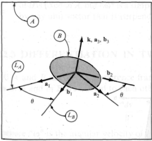
Figure 2.2.1

where \theta is theradianmeasure of the anglebetween aline L_{A} whose orientationis fixed in A andaline L_{B} similarlyfixed in B (seeFig.2.2.1),both lines are perpendicularto \mathbf{k} and \theta isregarded aspositivewhen the anglecanbegeneratedbyarotation of B relative to A duringwhich aright-handed screwrigidly attachedto B and parallel to \mathbf{k} advances in the direction of \mathbf{k} The scalarquantity \omega is called an angularspeedof B in A .The indefinite article“an”is usedhere because,if \tilde{\mathbf{k}} and \bar{\omega} are defined as {\dot{\mathbf{k}}}\ {\triangleq}\ -\mathbf{k} and \tilde{\omega}\triangleq-\omega then Eq. (1) can be written {}^{A}\mathbf{\Phi}\mathbf{(o)}^{B}=\tilde{\omega}\tilde{\mathbf{k}} so that \bar{\omega} is no less “the”angular speed than is .

Derivation Let \mathbf{a}_{1} \mathbf{a}_{2} \mathbf{a}_{3} bearight-handed set ofmutually erpendicular unit vectorsfixed in A with \mathbf{a}_{1} parallelto line L_{A} and {\bf a}_{3}={\bf k} and let {\mathfrak{b}}_{1} {\bf b}_{2} {\mathfrak{b}}_{3} bea similar set ofunitvectorsfixed in \boldsymbol{B} with \mathfrak{b}_{_{1}} parallelto L_{B} and \mathbf{b}_{3}=\mathbf{k}. Then

\begin{array}{r l}&{\mathbf{b}_{1}=\cos\theta\mathbf{a}_{1}+\sin\theta\mathbf{a}_{2}}\\ &{\mathbf{b}_{2}=-\sin\theta\mathbf{a}_{1}+\cos\theta\mathbf{a}_{2}}\\ &{\mathbf{b}_{3}=\mathbf{a}_{3}}\end{array}

{\frac{{}^{A}d{\bf b}_{1}}{d t}}=\dot{\theta}(-\sin\theta{\bf a}_{1}+\cos\theta{\bf a}_{2})=\dot{\theta}{\bf b}_{2}

\frac{^{A}d{\bf b}_{2}}{d t}=\dot{\theta}(-\cos\theta{\bf a}_{1}-\sin\theta{\bf a}_{2})=-\dot{\theta}{\bf b}_{1}

\frac{{}^{A}d{\bf b}_{3}}{d t}=0

and substitution into Eq.(2.1.1) leads directly to

{\bf{\nabla}}^{A}{\bf{e}}^{B}=\dot{\theta}{\bf{b}}_{3}=\dot{\theta}{\bf{k}}

Example Simple angular velocities are encountered most frequently in connectionwithbodies that aremeanttorotaterelativeto each other about axes fixedin thebodies,such as therotor and the gimbalrings ofagyroscope.This is illustrated inFig.2.2.2,whereA designates an aircraft that carries a gyroscope consisting of an outer gimbal B,an inner gimbal C,and a rotor D.Here,the angular velocities of Bin A,Cin B,and Din Call are simple angular velocities, and theycanbe expressed as

{}^{A}\!\upomega^{B}=\dot{q}_{1}\mathbf{b}\qquad\mathbf{\nabla}^{B}\!\upomega^{C}=\dot{q}_{2}\mathbf{c}\qquad\mathbf{\nabla}^{C}\!\upomega^{D}=-\dot{q}_{3}\mathbf{\dot{d}}

where q, q2, q3 measure angles as indicated in Fig. 2.2.2 and b, c, d are unt vectors directed as shown.(Note that,forexample,andarenot simple q_{3} \mathbf{d} angularvelociuies.) ArigidbodyBneednotbemountedinbearingsfixedin areference trame B Ain order tohave a simple angular velocity inA.Indeed,it is possiblefor B to have a simple angular velocity in A when B moves in such a way that no point of B remains fixed in A.For example,suppose that A is an aircraft in levelflight above a hillyroadway that liesin avertical plane,as depicted in Fig.2.2.3,and that Bis an automobile wheel traversing the roadway.No point of \pmb{B} is fixed in \pmb{A} ,but \pmb{A}_{\pmb{\omega}^{B}} is a simple angular velocity, the role of k being played by any unit vector that is perpendicular to the middle plane of the wheel.

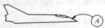
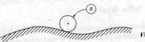
Figure 2.2.3

2.3 DIFFERENTIATION IN TWO REFERENCE FRAMES

If \pmb{A} and \pmb{B} are any two reference frames, the first time-derivatives of any vector \mathbf{y} in \pmb{A} and in \pmb{B} are related to each other as follows:

{\frac{{\boldsymbol{A}}_{d}\mathbf{v}}{d t}}={\frac{{\boldsymbol{B}}_{d}\mathbf{v}}{d t}}+{\boldsymbol{A}}_{\mathbf{0}}{\boldsymbol{^{B}}}\,\times\,\mathbf{v}

where \pmb{A_{\pmb{\omega}}}\pmb{B} is the angular velocity of \pmb{B} in \pmb{A} (see Sec. 2.1).

Derivation With \mathfrak{b}_{1},\mathfrak{b}_{2},\mathfrak{b}_{3} as in Sec. 2.1, let

v_{i}\triangleq\mathbf{v}\cdot\mathbf{b}_{i}\qquad(i=1,2,3)

so that [see Eqs. (1.3.1) and (1.3.2)]

\mathbf{v}=\sum_{i=1}^{3}v_{i}\mathbf{b}_{i}

Then

{\begin{array}{r l}&{{\frac{A_{d}\mathbf{v}}{d t}}={\frac{3}{\displaystyle\sum_{i=1}^{3}}}\ {\frac{d v_{i}}{d t}}\mathbf{b}_{i}+\sum_{i=1}^{3}v_{i}{\frac{d\mathbf{b}_{i}}{d t}}}\\ &{\qquad=\ {\frac{B_{d}\mathbf{v}}{d t}}\ +\ \sum_{i=1}^{3}v_{i}^{4}\mathbf{o}^{\ B}\ \mathbf{x}\ \mathbf{b}_{i}}\\ &{\qquad={\frac{B_{d}\mathbf{v}}{d t}}+\ A_{\mathbf{0}}^{\ B}\ \mathbf{x}\ \sum_{i=1}^{3}v_{i}\mathbf{b}_{i}}\\ &{\qquad={\frac{B_{d}\mathbf{v}}{d t}}+\ A_{\mathbf{0}}^{\ B}\ \mathbf{x}\ {\frac{\mathbf{0}}{t^{3}}}\ }\\ &{\qquad={\frac{B_{d}\mathbf{v}}{d t}}+\ A_{\mathbf{0}}^{\ B}\ \mathbf{x}\ \mathbf{v}}\\ &{\qquad\qquad\qquad\qquad\qquad\qquad\qquad\qquad\qquad\qquad\qquad\qquad\qquad\mathbf{0}}\end{array}}

Equation (1) enables one to find the time-derivative of \mathbf{y} in \pmb{A} without having to resolve \mathbf{v} into components parallel to unit vectors fixed in \pmb{A}

Example A vector \mathbf{H}_{} called the central angular momentum of a rigid body \pmb{B} in a reference frame A , can be expressed as

\mathbf{H}=I_{1}\omega_{1}\mathbf{b}_{1}+I_{2}\omega_{2}\mathbf{b}_{2}+I_{3}\omega_{3}\mathbf{b}_{3}

where \mathbf{b}_{1},\,\mathbf{b}_{2},\,\mathbf{b}_{3} form a certain set of mutually perpendicular unit vectors fixed in B,\omega_{j} is defined as

\omega_{j}\triangleq\omega^{B}\cdot\mathfrak{b}_{j}\qquad(j=1,2,3)

and I_{1},\,I_{2},\,I_{3} are constants, called central principal moments of inertia of \pmb{B}. With the aid of Eq. (1), one can find M_{1},M_{2} ， M_{3} such that the first timederivative of \mathbf{H} in \pmb{A} is given by

\frac{^{A}d{\bf H}}{d t}=M_{1}{\bf b}_{1}+M_{2}{\bf b}_{2}+M_{3}{\bf b}_{3}

Specifically,

\begin{array}{r l}{\displaystyle\frac{\ensuremath{\boldsymbol}{A}_{\mathrm{{H}}}}{\ensuremath{\boldsymbol}{d t}}}&{=}&{\displaystyle\frac{\ensuremath{\boldsymbol}{B}_{d\mathrm{H}}}{\ensuremath{\boldsymbol}{d t}}+\iota_{0}\boldsymbol{\theta}^{\phantom{\dagger}}\times\mathrm{\boldmath{~H~}}}\\ {\displaystyle\frac{\ensuremath{\boldsymbol}{a}_{d\mathrm{H}}}{\ensuremath{\boldsymbol}{d t}}}&{=}&{I_{1}\dot{\omega}_{1}\dot{\ensuremath{\mathbf{b}}}_{1}+I_{2}\dot{\omega}_{2}\dot{\ensuremath{\mathbf{b}}}_{2}+I_{3}\dot{\omega}_{3}\dot{\ensuremath{\mathbf{b}}}_{3}}\\ {\displaystyle\dot{\iota}_{0}\boldsymbol{\theta}}&{=}&{\displaystyle\omega_{1}\dot{\ensuremath{\mathbf{b}}}_{1}+\omega_{2}\dot{\ensuremath{\mathbf{b}}}_{2}+\omega_{3}\dot{\ensuremath{\mathbf{b}}}_{3}}\\ {\displaystyle\dot{\iota}_{0}\boldsymbol{\theta}}&{=}&{\displaystyle(\omega_{2}I_{3}\omega_{3}-\omega_{3}I_{2}\omega_{2})\dot{\ensuremath{\mathbf{b}}}_{1}+\cdots}\\ {\displaystyle\frac{\ensuremath{\boldsymbol}{A}_{d\mathrm{H}}}{\ensuremath{\boldsymbol}{d t}}}&{=}&{\displaystyle[I_{1}\dot{\omega}_{1}-(I_{2}-I_{3})\omega_{2}\omega_{3}]\dot{\ensuremath{\mathbf{b}}}_{1}+\cdots}\end{array}

It follows from Eqs. (7) and (12) that

\begin{array}{r}{M_{1}=I_{1}\dot{\omega}_{1}-\left(I_{2}-I_{3}\right)\omega_{2}\omega_{3}}\\ {M_{2}=I_{2}\dot{\omega}_{2}-\left(I_{3}-I_{1}\right)\omega_{3}\omega_{1}}\\ {M_{3}=I_{3}\dot{\omega}_{3}-\left(I_{1}-I_{2}\right)\omega_{1}\omega_{2}}\end{array}

2.4 AUXILIARY REFERENCE FRAMES

The angular velocity of a rigid body \pmb{B} in a reference frame \pmb{A} (see Sec. 2.1) can be expressed in the following form involving \pmb{n} auxiliary reference frames A_{1},...,A_{n}

A_{\dot{\mathbf{O}}}{}^{B}\,=\,A_{\dot{\mathbf{O}}}A_{1}\,+\,A_{1}}_{\dot{\mathbf{O}}}A_{2}\,+\,\cdot\,\cdot\,+\,A_{n-1}_{\dot{\mathbf{O}}}A_{n}\,+\,A_{n}_{\dot{\mathbf{O}}}B

This relationship, the addition theorem for angular velocities, is particularly useful when each term in the right-hand member represents a simple angular velocity (see Sec. 2.2) and can, therefore, be expressed as in Eq. (2.2.1). However, Eq. (1) applies even when one or more of \pmb{\mathscr{A}}_{\pmb{\mathscr{G}}\pmb{\mathscr{D}}}\pmb{\mathscr{A}}_{1} \pmb{A}_{n_{0},\pmb{B}} are not simple angular velocities.

Thereference frames A_{1},...,A_{n} may or may not correspond to actual rigid bodies. Frequently, such reference frames are introduced as aids in analysis, but have no physical counterparts.

When the angular velocity of \pmb{B} in \pmb{A} is resolved into components (that is, when \pmb{A_{\mathbb{Q}^{\pmb{\beta}}}} is expressed as the sum of a number of vectors), these components may always be regarded as angular velocities of certain bodies in certain reference frames. Indeed, Eq. (1) represents precisely such a resolution of \pmb{A}_{\pmb{\omega}}\pmb{B} into components. In no case, however, are these components themselves angular velocities of \pmb{B} in \pmb{A} , for there exists at any one instant only one angular velocity of \pmb{B} in \pmb{A} . In other words, \pmb{B} cannot possess simultaneouslyt several angular velocities in \pmb{A}

Derivation For any vector \upbeta fxed in \pmb{B}

\begin{array}{l}{{{\displaystyle\frac{{}A{\cal\/}8}{d t}~~=~~{}^{A}{\bf\omega}^{B}{}~\times~\beta}}}\\ {{{\displaystyle\frac{{}A{}_{1}}{d t}{}_{(2,1,2)}}{}}}\end{array}\!\!\!\!\!\!\!\!\!\!\!\!\!\!\!\!\!\!\!\!\!\!\!\!\!\!\!\!{\displaystyle\frac{A_{1}}{d t}{}_{(2,1,2)}}={}\!\!\!\!\!\!\!\!\!\!\!{A_{1}}{}_{(0)}{}^{B}{}~\times{}~\beta

and

\frac{^{A}\!d{\mathbb{B}}}{d t}_{(2.3.1)}\frac{^{A_{1}}d{\mathbb{B}}}{d t}+\!\!\!\nabla\!\!\Theta^{A_{1}}\times{\mathbb{B}}

Hence,

A_{\bigstar}{}^{B}\times{}~\beta={}^{A_{1}}{}_{\bigstar}{}^{B}\times{}^{\beta}+{}^{A}{\mathfrak{W}}^{A_{1}}\times{}^{\beta}

Since this equation is satisfied by every \pmb{\upbeta} fixed in \pmb{B}. it implies that

^{A}\!\mathbf{\omega}\!\mathbf{\omega}^{B}={\^{A}\!\mathbf{\omega}\!\mathbf{\omega}^{A_{1}}}+{^{A_{1}}\!\mathbf{\omega}\!\mathbf{\omega}^{B}}

which shows that Eq. (1) is valid for n=1 Proceeding similarly, one can verify that

A_{1}}_{\underline{{{\Theta}}}}B\,=\,A_{1}_{\underline{{{\Theta}}}}A_{2}\,+\,A_{2}_{\underline{{{\Theta}}}}B

and substitution into Eq. (6) then yields

A_{\dot{\Theta}}B\,=\,A_{\dot{\Theta}}A_{1}\,+\,A_{1}_{\dot{\Theta}}A_{2}\,+\,A_{2}_{\dot{\Theta}}B

which is Eq. (1) with n=2. The validity of Eq. (1) for any value of \pmb{n} thus can be established by applying this procedure a suffcient number of times.

Example In Fig. 2.4.1, q_{1},\,q_{2} , and \pmb q_{3} denote the radian measures of angles characterizing the orientation of a rigid cone \pmb{B} in a reference frame A. These angles are formed by lines described as follows: L_{1} and L_{2} are perpendicular to each other and fixed in A;L_{3} is the axis of symmetry of \pmb{B} \scriptstyle L_{4} is perpendicular to L_{2} and intersects L_{2} and L_{3}\colon L_{5} is perpendicular to L_{3} and intersects L_{2} and L_{3}\colon L_{6} is perpendicular to L_{3} and is fixed in B;L_{7} is perpendicular to L_{2} and L_{4} . To find an expression for the angular velocity of \pmb{B} in \pmb{A} , one can designate as A_{1} a reference frame in which L_{2},L_{4} . and L_{7} are fixed, and as A_{2} a reference frame in which L_{3},L_{5} , and L_{7} are fixed, observing that L_{2}

^{\dagger} In the literature, one encounters not infrequently the equation {\bf\omega}_{0}={\bf\omega}_{0},+{\bf\omega}_{0}, , accompanied bya discussion of“simultaneous angular velocities of arigid body" andor“the vector character of angular velocity." Moreover, \mathbf{\omega_{0}} and {\bf\omega}_{0} often are called angular velcities of \pmb{{\cal B}} about certain axes. This eadsontwnderwmanysuhaxeexist inagivease,hwncanlocate hmando forththtfanllitbt naxisrfsl to dispense with it.

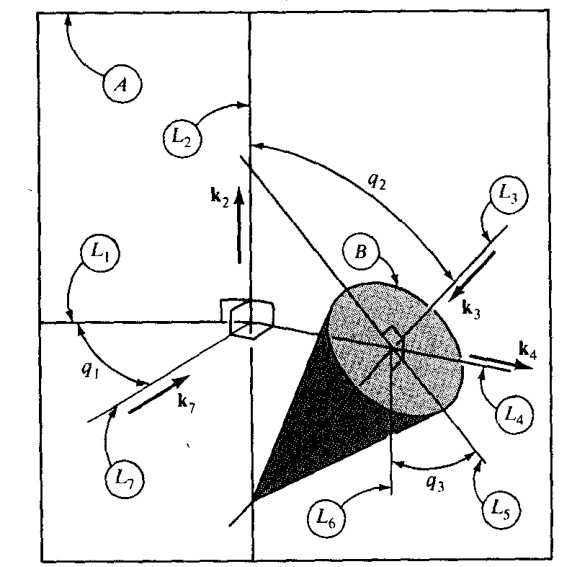
Figure 2.4.1

then is fixed both in A and A_{1},L_{7} is fixed both in A_{1} and A_{2} , and L_{3} is fixed bothin A_{2} and B , so that, in accordance with Eqs. (2.2.1) and (2.2.2), one can write

{}^{A}\!\Theta^{A_{1}}=\dot{q}_{1}{\bf k}_{2}\qquad{}^{A_{1}}\!\Theta^{A_{2}}=\dot{q}_{2}{\bf k}_{7}\qquad{}^{A_{2}}\!\Theta^{B}=\dot{q}_{3}\,{\bf k}_{3}

where k2, k7, and k, are unit vectors directed as shown in Fig. 2.4.1. Substituting from Eq. (9) into Eq. (1) with n=2 onearrivesat

A_{\bf0}{}^{B}=\dot{q}_{1}{\bf k}_{2}+\dot{q}_{2}{\bf k}_{7}+\dot{q}_{3}{\bf k}_{3}

2.5 ANGULAR ACCELERATION

The angular acceleration Aa of a rigid body B in a reference frame A is defined as the first time-derivative in A of the angular velocity of B in A (see Sec. 2.1):

A_{\mathfrak{A}}{}^{B}\triangleq\frac{{}^{A}d^{A}\mathfrak{A}^{B}}{d t}

Since the first time-derivatives of \mathbf{\mathit{A}}_{\mathbf{\Theta}\mathbf{\tilde{0}}}\mathbf{\mathit{B}} in \pmb{A} andin B are equal toeach other, as becomes evident when one replaces v in Eq. (2.3.1) with 4o", Eq. (1) implies that

A_{\mathfrak{A}}B=\frac{B_{d}A_{\mathfrak{A}}^{B}}{d t}

which furnishes a convenient way to find AaB when Ao3 has been expressed in terms of components parallel to unit vectors fixed in \boldsymbol{B}

If A_{1},...,A_{n} are n auxiliary reference frames, A_{\alpha}B is not, in general, equal to the sum \mathbf{\dot{\alpha}}^{A}\mathbf{\alpha}^{A_{1}}+\mathbf{\alpha}^{A_{1}}\mathbf{\alpha}^{A_{2}}+\mathbf{\beta}^{\dots}+\mathbf{\alpha}^{A_{n}}\mathbf{\alpha}^{B} . Thus, Eq. (2.4.1) does not, in general, have an angular acceleration counterpart.

The angular velocity of \boldsymbol{B} in A can always be expressed as {}^{A}\mathbf{\omega}\mathbf{\omega}^{B}=\omega\mathbf{k}_{\omega} , where \mathbf{k}_{\omega} is a unit vector parallel to \mathbf{\mathit{A}_{G D}}\mathbf{\mathit{B}} ; similarly A_{\widetilde{\mathbf{z}}}B can always be expressed as ^{A}\pmb{\alpha}^{B}=\alpha\mathbf{k}_{\alpha} , where \mathbf{k}_{\alpha} is a unit vector parall to A_{\pmb{\alpha}}B In general, \mathbf{k}_{\omega} differs from \mathbf{k}_{\alpha} ， and \alpha\neq d\omega/d t . But when \boldsymbol{B} has a simple angular velocity in A (see Sec. 2.2), and \mathbf{\Pi}^{A}\mathbf{\Pi}_{\mathbf{G}\mathbf{\tilde{D}}}\mathbf{\scriptscriptstyle{B}} is expressed as in Eq. (2.2.1), then

A_{\alpha}B_{\mathrm{\Phi}}={\mathfrak{X}}\mathbf{k}

where \pmb{\alpha}_{\ast} called a scalar angular acceleration, is given by

\alpha={\frac{d\omega}{d t}}

Example Referring to the example in Sec. 2.4 and to Fig. 2.4.1, one can find an expression for the angular acceleration of the cone \pmb{B} inreferenceframe \pmb{A} asfollows:

{\begin{array}{r l}&{{\mathbf{\nabla}}_{a{\pmb{\alpha}}^{B}}={\cfrac{a_{d}}{d t}}({\dot{q}}_{1}{\mathbf{k}}_{2}+{\dot{q}}_{2}{\mathbf{k}}_{7}+{\dot{q}}_{3}{\mathbf{k}}_{3})}\\ &{\qquad={\ddot{q}}_{1}{\mathbf{k}}_{2}+{\dot{q}}_{1}{\cfrac{a_{d}{\mathbf{k}}_{2}}{d t}}+{\ddot{q}}_{2}{\mathbf{k}}_{7}+{\dot{q}}_{2}{\cfrac{a_{d}{\mathbf{k}}_{7}}{d t}}+{\ddot{q}}_{3}{\mathbf{k}}_{3}+{\dot{q}}_{3}{\cfrac{a_{d}{\mathbf{k}}_{3}}{d t}}}\end{array}}\,,{\mathbf{\dot{\xi}}}_{{\begin{array}{r}{{\dot{\mathbf{\xi}}}_{{\mathrm{~f~i~s~}}^{A}}\end{array}}}}\,,{\mathbf{\dot{\xi}}}_{{\begin{array}{r}{{\dot{\mathbf{\xi}}}_{{\mathrm{~f~i~s~}}^{A}}\end{array}}}}\,,

Since \mathbf{k}_{2} is fixed in A

\frac{{}^{A}d{\bf k}_{2}}{d t}=0

The unit vector \mathbf{k}_{7} is fixed in a reference frame previously called A_{1} and having an angular velocity in A given by

\begin{array}{r l r}{{}^{A}\pmb{\omega}^{A_{1}}}&{{}=}&{\dot{q}_{1}\pmb{\mathrm{k}}_{2}}\end{array}

Hence,

\frac{^{A}d\mathbf{k}_{7}}{d t}=\mathbf{\nabla}_{(2.1.2)}^{A}\mathbf{\omega}\mathbf{\omega}^{A_{1}}\times\mathbf{k}_{7}=\dot{q}_{1}\mathbf{k}_{2}\times\mathbf{k}_{7}

Similarly, since {\bf k}_{3} is fixed in \pmb{B}_{\pmb{\cdot}}

\frac{{^A\!\!\!\!/}k_{3}}{d t}={^A\!\!\!\!/}\mathfrak{w}^{B}\times\,{\bf k}_{3}\qquad=\qquad\dot{q}_{1}{\bf k}_{2}\times{\bf k}_{3}^{\quad\cdot}+\dot{q}_{2}{\bf k}_{7}\times{\bf k}_{3}

Consequently,

\begin{array}{r l}{\lefteqn{^{A}\!\!{\pmb\alpha}^{B}=\ddot{q}_{1}{\bf k}_{2}+0+\ddot{q}_{2}{\bf k}_{7}+\dot{q}_{2}\dot{q}_{1}{\bf k}_{2}\times{\bf k}_{7}}}\\ &{\quad\quad+\ddot{q}_{3}{\bf k}_{3}+\dot{q}_{3}(\dot{q}_{1}{\bf k}_{2}\times{\bf k}_{3}+\dot{q}_{2}{\bf k}_{7}\times{\bf k}_{3})}\end{array}

The angular accelerations of A_{1} in A,A_{2} in A_{1} , and \pmb{B} in A_{2} are

{}^{A}\!\!\!\alpha^{A_{1}}={\frac{{}^{A}\!\!d^{A}\!\!\omega^{A_{1}}}{d t}}=\ddot{q}_{1}\mathbf{k}_{2}

A_{1}{\bf q}^{A_{2}}=\frac{{\cal A}_{1}}{d t}{\bf\Gamma}_{(2.4.9)}=\mathrm{~\Gamma~}_{\!\!\{2.4.9\}}\!\!\!\!\!\!\!\!\!\!\!\!\!\!\!\!\!\!\!\!\!\!\!\!\!\!\!\!\!\!\!\!\!\!\!\!\!\!\!\!\!\!\!\!\!\!\!\!\!\!\!\!\!\!\!\!\!\!\!\!\!\!\!\!\!\!\!\!\!\!\!\!\!\!\!\!\!\!\!\!\!\!\!\!\!\!\!\!\!\!\!\!\!\!\!\!\!\!\!\!\!\!\!\!\!\!\!\!\!\!\!\!\!\!\!\!\!\!\!\!\!\!\!\!\!\!\!\!\!\!\!\!\!\!\!\!\!\!\!\!\!\!\!\!\!\!\!\!\!\!\!\!\!\!\!\!\!\!\!\!\!\!\!\!\!\!\!\!\!\!\!\!\!\!\!\!\!\!\!\!\!\!\!\!\!\!\!\!\!\!\!\!\!\!\!\!\!\!\!\!\!\!\!\!\!\!\!\!\!\!\!\!\!\!\!\!\!\!\!\!\!\!\!\!\!\!\!\!\!\!\!\!\!\!\!\!\!\!\!\!\!\!\!\!\!\!\!\!\!\!\!\!\!\!\!\!\!\!\!\!\!\!\!\!\!\!\!\!\!\!\!\!\!\!\!\!\!\!\!\!\!\!\!\!\!\!\!\!\!\!\!\!\!\!\!\!\!\!\!\!\!\!\!\!\!\!\!\!\!\!\!\!\!\!\!\!\!\!\!\!\!\!\!\!\!\!\!\!\!\!\!\!\!\!\!\!\!\!\!\!\!\!\!\!\!\!\!\!\!\!\!\!\!\!\!\!\!\!\!\!\!\!\!\!\!\!\!\!\!\!\!\!\!\!\!\!\!\!\!\!\!\!\!\!\!\!\!\!\!\!\!\!\!\!\!\!\!\!\!\!\!\!\!\!\!\!\!\!\!\!\!\!\!\!\!\!\!\!\!\!\!\!\!\!\!\!\!\!\!\!\!\!\!\!\!\!\!\!\!\!\!\!\!\!\!\!\!\!\!\!\!\!\!\!\!\!\!\!\!\!\!\!\!\!\!\

A_{^2{\pmb{\alpha}}}{\pmb{\alpha}}^{B}=\frac{a_{^2}d^{A_{^2}}{\pmb{\omega}}^{B}}{d t}=\underset{(2.4.9)}{\ddot{q}}_{3}\,{\bf k}_{3}

Hence,

{}^{A}\!\!\!\!\alpha^{A_{1}}\,+\,{}^{A_{1}}\!\!\!\alpha^{A_{2}}\,+\,{}^{A_{2}}\!\!\!\alpha^{B}=\,\ddot{q}_{1}\mathbf{k}_{2}\,+\,\ddot{q}_{2}\,\mathbf{k}_{7}\,+\,\ddot{q}_{3}\,\mathbf{k}_{3}\,\neq\,{}^{A}\!\!\!\alpha^{B}

2.6 VELOCITY AND ACCELERATION

The solution of nearly every problem in dynamics requires the formulation of expressions for velocities and accelerations of points of a system under consideration. At times, the most convenient way to generate the needed expressions is to use the definitions given below. Frequently, however, much labor can be saved by appealing to the theorems ^{\dagger} stated in Secs. 2.7 and 2.8.

Let p denote the position vector from any point o fixed in a reference frame \pmb{A} to a point P moving in A . The velocity of P in A and the acceleration of P in A ， denoted by \pmb{A}_{\mathbf{v}}\pmb{P} and A_{\mathbf{a}}P , respectively, are defined as

A_{\mathbf{v}}P\triangleq{\frac{4}{d t}}

and

A_{\mathfrak{a}}P\triangleq{\frac{\mathfrak{A}d^{A}\mathbf{v}^{P}}{d t}}

Example In Fig. 2.6.1, P_{1} and P_{2} designate two points connected by a line of length \pmb{L} and free to move in a plane \pmb{B} that is rotating at a constant rate \omega about a line \pmb{Y} fixed both in \pmb{B} and in a reference frame A. The velocities \pmb{A}_{\mathbf{y}}\pmb{P}_{\mathbf{l}} and A_{\mathbf{v}}P_{2} of \boldsymbol{P}_{1} and \boldsymbol{P}_{2} in A are to be expressed in terms of the quantities q_{1},\,q_{2},\,q_{3} , their time-derivatives \dot{q}_{1},\,\dot{q}_{2},\,\dot{q}_{3} , and the mutually perpendicular unit vectors \pmb{\mathrm{e}}_{x},\pmb{\mathrm{e}}_{y},\pmb{\mathrm{e}}_{z} shown in Fig. 2.6.1.

^\dagger The discussion of velocities and accelerations in Secs. 2.7 and 2.8 involves the concept of angular velocity. Hence, to come into position to present this material without a break in continuity, one must deal with angular velocity before taking up velocity and acceleration. Conversely, as Secs. 2.1-2.4 show, angular velocity can be discussed without any reference to velocity or acceleration. Therefore, it is both natural and advantageous to treat these topics in the order used here, that is, angular velocity before velocity and acceleration, rather than in the reverse order.

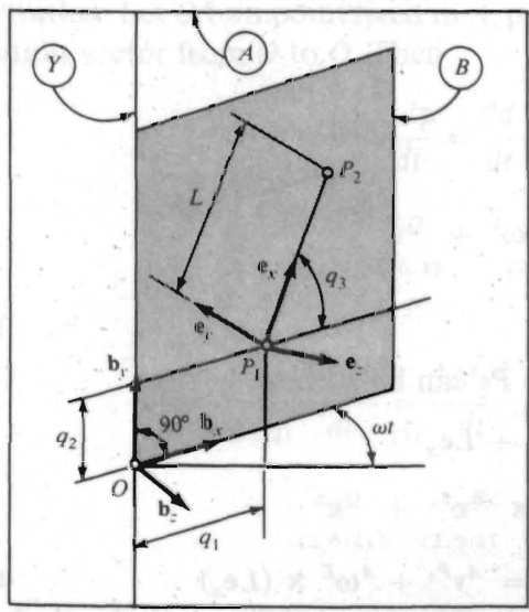
Figure 2.6.1

Thepoint o shown inFig.2.6.1is a point fixed in A_{i} andthepositionvector {\bf p}_{1} from o to {\dot{P}}_{1} canbewritten

\mathbf{p}_{1}=q_{1}\mathbf{b}_{x}+q_{2}\mathbf{b}_{y}

where \mathbf{b}_{x} and {\bf b}_{y} are unit vectors directed as shown inFig.2.6.1.Itfollows that

A_{\bf{V}}^{P_{1}}=\frac{{\displaystyle{{\cal A}}_{{\bf{P}}_{1}}}}{d t}{\displaystyle{\sum_{(2,3,1)}}^{2}}{\displaystyle{\frac{{\displaystyle{{\cal B}}}_{d{\bf{P}}_{1}}}{d t}}}+{\displaystyle{{\cal A}_{0}}^{B}}\times{\bf{\nabla}}{{\bf p}_{1}}

where

\frac{{\mathop{B}}d{\mathbf{p}}_{1}}{d t}=\dot{q}_{1}{\mathbf{b}}_{x}+\dot{q}_{2}{\mathbf{b}}_{y}

and

{\bf{\nabla}}^{A}\Phi^{B}\times\,{\bf{p}}_{1}\,=\,\omega{\bf{b}}_{y}\,{\bf{\nabla}}\times\,(q_{1}{\bf{b}}_{x}\,+\,q_{2}\,{\bf{b}}_{y})=\,-\,\omega q_{1}{\bf{b}}_{z}

so that

\begin{array}{r}{{\bf\nabla}^{A}{\bf v}^{P_{1}}=\dot{q}_{1}{\bf b}_{x}+\dot{q}_{2}{\bf b}_{y}-\omega q_{1}{\bf b}_{z}}\\ {{\bf\nabla}^{(4)}~~~~~~~~~~~~~~~(6)\mathrm{~\boldmath~\Omega~}}\end{array}

Since the unit vectors \mathfrak{b}_{x} {\bf b}_{y} \mathfrak{b}_{z} are related to the unit vectors \mathbf{e}_{x} \mathbf{e}_{y} \mathbf{e}_{z} as in Table 2.6.1, where {\bf s}_{3} and \mathbf{c}_{3} stand for sin q_{3} and cos q_{3} ,respectively, Eq. (7) is equivalent to

{\bf\nabla}^{A}{\bf v}^{P_{1}}=(\dot{q}_{1}{\sf c}_{3}+\dot{q}_{2}{\sf s}_{3}){\bf e}_{x}+(-\dot{q}_{1}{\bf s}_{3}+\dot{q}_{2}{\sf c}_{3}){\bf e}_{y}-\omega q_{1}{\bf e}_{z}

which is the desired expression for the velocity of \boldsymbol{P}_{1} in _{A}

Table 2.6.1

<html>

	e.x	ey	ez
bx	C3	- S3	0
by	$3	C3	0
bz	0	0	1

</html>

The position vector \begin{array}{r}{\pmb{\mathsf{p}}_{2}}\end{array} from o to P_{2} can be written

{\bf p}_{2}={\bf p}_{1}+L{\bf e}_{x}

Hence,

A_{\mathbf{V}^{P_{2}}}={\frac{{\mathit{A}}d_{\mathbf{\overline{{p}}}_{1}}}{d t}}+{\frac{{\mathit{A}}d}{d t}}(L\mathbf{e}_{x})={\mathit{\omega}}_{(4)}^{A}P_{1}^{P_{1}}+{\mathit{\omega}}_{(4)}^{A}{\mathit{\omega}}\times(L\mathbf{e}_{x})

where \mathbf{\Delta}_{\mathbf{G}\mathbf{\tilde{D}}}\mathbf{\tilde{E}} is the angular velocity in A of a rigid body E in which \pmb{\mathrm{e}}_{x},\pmb{\mathrm{e}}_{y},\pmb{\mathrm{e}}_{z} are fixed ; that is,

\begin{array}{c}{{{\bf\Gamma}^{A}{\bf\omega}^{E}\mathrm{\boldmath~\omega~}=\mathrm{\boldmath~\Gamma~}^{A}{\bf\omega}^{B}+\mathrm{\boldmath~\cal~}^{B}{\bf\omega}^{E}=\mathrm{\boldmath~\omega~}\omega{\bf b}_{y}\mathrm{\boldmath~\omega~}+\mathrm{\boldmath~\dot{q}~}_{3}{\bf b}_{z}}}\\ {{\mathrm{\boldmath~\Gamma~}^{(2.4.1)}\mathrm{\boldmath~\Gamma~}^{(3)}}}\\ {{\mathrm{\boldmath~\Gamma~}\mathrm{\boldmath~\omega~}=\mathrm{\boldmath~\omega~}\omega s_{3}\,{\bf e}_{x}+\omega c_{3}{\bf e}_{y}+\dot{q}_{3}{\bf e}_{z}}}\\ {{\mathrm{\boldmath~\Gamma~}^{(\mathrm{Table}}}}\\ {{\mathrm{\boldmath~\Gamma~}^{2.6.1)}}}\end{array}

so that

{}^{A}\!\upomega^{E}\,\times\,(L\mathbf{e}_{x})\,=\,L(\dot{q}_{3}\,\mathbf{e}_{y}\,-\,\omega c_{3}\,\mathbf{e}_{z})

and

\begin{array}{r l r}{{^A_{\bf v}}{^P}_{^2}}&{{}=}&{(\dot{q}_{1}c_{3}+\dot{q}_{2}s_{3}){\bf e}_{x}+(-\dot{q}_{1}s_{3}+\dot{q}_{2}c_{3}+L\dot{q}_{3}){\bf e}_{y}-\omega(q_{1}+L c_{3}){\bf e}_{z}}\end{array}

2.7 TWO POINTS FIXED ON A RIGID BODY

If P and Q are two points fixed on a rigid body \pmb{B} having an angular velocity \mathbf{\Omega_{op}}^{B} in \pmb{A} , then the velocity \pmb{A}_{\mathbf{v}}\pmb{P} of \pmb{P} in \pmb{A} and the velocity \pmb{A}_{\mathbf{v}}\pmb{Q} of Q in \pmb{A} are related to each other as follows:

^{A}\mathbf{v}^{P}={^{A}\mathbf{v}^{Q}}+{^{A}\!\mathbf{\omega}^{B}}\times\mathbf{r}

where r is the position vector from Q to \pmb{P} . The relationship between the acceleration A_{\mathbf{a}}P of \pmb{P} in \pmb{A} and the acceleration \pmb{a}_{\mathbf{a}}\pmb{Q} of Q in \dot{\pmb{A}} involves the angular acceleration A_{\pmb{\alpha}}B of \pmb{B} in \pmb{A} and is given by

{}^{A}{\pmb a}^{P}={}^{A}{\pmb a}^{Q}+{}^{A}{\pmb\omega}^{B}\times({}^{A}{\pmb\omega}^{B}\times{}\,{\bf r})\,+\,{}^{A}{\pmb\alpha}^{B}\,\times\,{}^{\bf r}

Derivation Let ^o be a point fixed in A,\mathfrak{p} the position vector from o to \pmb{P} and \mathfrak{q} the position vector from ^o to Q . Then

\begin{array}{c}{{{\cal A}_{\bf v}P\mathrm{\boldmath~\omega~}=\mathrm{\boldmath~\displaystyle\frac{\calA}{\cal d t}~}{\cal\dot{\Pi}}=\displaystyle\frac{\cal A}{d t}({\bf q}+{\bf r})=\displaystyle\frac{{\cal A}_{d{\bf q}}}{d t}+\frac{{\cal A}_{d{\bf r}}}{d t}}}\\ {{\mathrm{\boldmath~\mu~}=\mathrm{\boldmath~\displaystyle~\calA_{\bfv}Q~}+{\cal A}_{\bf0}{\bf^{B}\times r}}}\end{array}

and

\begin{array}{c}{{\displaystyle{\bf\cal A}_{\bf\underline{{{a}}}^{P}{\bf\Pi}}_{(2.6.2)}={\frac{A_{d}A_{\bf{v}^{P}}}{d t}}={\frac{A_{d}A_{\bf{v}^{Q}}}{d t}}+{\frac{A_{d}A_{\bf{\omega}^{B}}}{d t}}\times{\bf\Gamma}+\bf{\Gamma}^{A}{\bf\omega}^{B}\times{\frac{A_{d}{\bf r}}{d t}}}}\\ {{\displaystyle={\operatorname*{\boldmath}\omega}_{(2.6.2)}{\bf\Gamma}_{(2.5.1)}^{A_{\bf{\bar{a}}^{Q}}}\times{\bf\Gamma}{\bf r}+{\bf\Gamma}^{A}{\bf\omega}^{B}\times({\bf\Gamma}^{A}{\bf\omega}^{B}\times{\bf\Gamma})}}\end{array}

Example Since an expression for the velocity of \boldsymbol{P}_{1} in \pmb{A} in the example in Sec. 2.6 is available in Eq. (2.6.7), the acceleration of \boldsymbol{P}_{1} in \pmb{A} can be found most directly by differentiating this expression, which yields

\begin{array}{r l}{\displaystyle{^{A}\mathfrak{a}^{P_{1}}}_{(2,6,2)}\frac{\mathfrak{a}_{d}^{A}\mathfrak{v}^{P_{1}}}{d t}\qquad\displaystyle=\frac{\mathfrak{a}_{d}^{B}\mathfrak{v}^{P_{1}}}{d t}+\,^{A}\mathfrak{a}^{B}\times\,^{A}\mathfrak{v}^{P_{1}}}\\ {\displaystyle{^{(2,6,2)}}\qquad\mathfrak{a}_{1}^{-}+\,\ddot{\mathfrak{a}}_{2}^{-}\mathfrak{b}_{3}\ -\omega\dot{\mathfrak{q}}_{1}\mathfrak{b}_{z}\,+\,\omega\mathfrak{b}_{\mathfrak{y}}\ \times\,^{A}\mathfrak{v}^{P_{1}}}\\ {\displaystyle\qquad=\ (\ddot{\mathfrak{q}}_{1}\mathfrak{b}_{x}+\,\dot{\mathfrak{q}}_{2}\mathfrak{b}_{y})}\\ {\displaystyle{^{(2,6,7)}}\qquad\qquad\qquad\qquad\qquad\qquad\qquad\qquad\qquad\qquad\qquad\,^{(2,2,1)}}\end{array}

In the case of \boldsymbol{P}_{2} , it is more convenient to use Eq. (2) together with the result just obtained than it is to difrentiate the expression for \pmb{{A}}_{\mathbf{y}}\pmb{{P}}_{2} available in Eq. (2.6.13). Letting P_{1} and \scriptstyle P_{2} play the parts of \b{Q} and \pmb{P} , respectively, in Eq. (2), and replacing \pmb{B} with E , since \boldsymbol{P}_{1} and \boldsymbol{P}_{2} are fixed on {\pmb E} , not on \pmb{B} one can write

{}^{A}\mathbf{a}^{P_{2}}={}^{A}\mathbf{a}^{P_{1}}+{}^{A}\mathbf{\omega}^{E}\times[{}^{A}\mathbf{\omega}\mathbf{\omega}^{E}\times(L\mathbf{e}_{x})]+{}^{A}\mathbf{\omega}^{E}\times(L\mathbf{e}_{x})

Now,

\begin{array}{r}{^{A}\!\!\odot^{E}\times\,[^{A}\!\!\odot^{E}\times(L\mathbf e_{x})]\qquad\qquad=\qquad\!\!L[-(\omega^{2}{\bf c}_{3}^{\,2}+\,\dot{q}_{3}^{\,2})\mathbf e_{x}}\\ {(2.6.11,2.6.12)\qquad\qquad\qquad\qquad\qquad\qquad\qquad+\,\omega^{2}s_{3}\,\mathbf c_{3}\mathbf e_{y}+\omega\dot{q}_{3}\,s_{3}\mathbf e_{z}]}\end{array}

and

{^A\!\!\!{\pmb{\alpha}}}_{(2.5.2)}^{E}\frac{{^E\!\!d}_{0}^{A}{\bf0}^{E}}{d t}{^{\!\!\!{\frac{1}{2}}}}_{(2.6.11)}\omega\dot{q}_{3}{\bf c}_{3}{\bf e}_{x}-\omega\dot{q}_{3}s_{3}{\bf e}_{y}+\ddot{q}_{3}{\bf e}_{z}

so that

\mathbf{\Psi}^{A}\pmb{\alpha}^{E}\,\times\,(L\pmb{e}_{x})=L(\ddot{q}_{3}\pmb{\mathrm{e}}_{y}+\omega\dot{q}_{3}\,\mathbf{s}_{3}\,\mathbf{e}_{z})

Substitution from Eqs. (5), (7), and (9) into Eq. (6) yields

\begin{array}{r}{\mathbf{\nabla}^{A}\mathbf{\bar{a}}^{P_{2}}=(\ddot{q}_{1}-\omega^{2}q_{1})\mathbf{b}_{x}+\ddot{q}_{2}\mathbf{b}_{y}-2\omega(\dot{q}_{1}-L\dot{q}_{3}\mathbf{\{s}}_{3})\mathbf{b}_{z}}\\ {+\mathbf{\nabla}L[-(\omega^{2}{\mathbf{c_{3}}}^{2}+\dot{q}_{3}{}^{2})\mathbf{e}_{x}+(\omega^{2}\mathbf{s}_{3}\mathbf{c}_{3}+\ddot{q}_{3})\mathbf{e}_{y}]}\end{array}

If one wishes to express this vector solely in terms of \begin{array}{r}{\mathbf{b}_{x},\mathbf{b}_{y},\mathbf{b}_{z}}\end{array} , one can refer to Table 2.6.1 to obtain

\begin{array}{r l}&{^{A}\mathbf{a}^{P_{2}}=[\ddot{q}_{1}-\omega^{2}q_{1}-L(\ddot{q}_{3}\mathfrak{s}_{3}+{\dot{q}_{3}}^{2}\mathfrak{c}_{3}+\omega^{2}\mathfrak{c}_{3})]\mathbf{b}_{\boldsymbol{x}}}\\ &{\qquad\quad+\mathbf{\nabla}[\ddot{q}_{2}+L(\ddot{q}_{3}\mathfrak{c}_{3}-{\dot{q}_{3}}^{2}\mathfrak{s}_{3})]\mathbf{b}_{\boldsymbol{y}}-2\omega(\dot{q}_{1}-L\dot{q}_{3}\mathfrak{s}_{3})\mathbf{b}_{\boldsymbol{z}}}\end{array}

2.8 ONE POINT MOVING ON A RIGID BODY

If a point \pmb{P} is moving on a rigid body \pmb{B} while \pmb{B} is moving in a reference frame \pmb{A} the velocity \pmb{A}_{\mathbf{v}}\pmb{P} of \pmb{P} in \pmb{A} is related to the velocity \pmb{{\cal B}}_{\mathbf{v}}\pmb{{\cal P}} of \pmb{P} in \pmb{B} as follows:

A_{\mathbf{v}}P\,=\,A_{\mathbf{v}}\bar{B}\,+\,B_{\mathbf{v}}P

where \pmb{A}_{\mathbf{v}}\pmb{\breve{B}} denotes the velocity in \pmb{A} of the point \bar{\pmb{B}} of \pmb{B} that coincides with P at the instant under consideration. The acceleration \pmb{A}_{\pmb{\mathscr{a}}}\pmb{P} of \pmb{P} in \pmb{A} isgiven by

A_{\mathbf{a}}P\,=\,A_{\mathbf{a}}{}^{B}\,+\,{}^{B}{\mathbf{a}}^{P}\,+\,2^{A}{\mathbf{\omega}}^{B}\,\times\,{}^{B}{\mathbf{v}}^{P}

where A_{\mathbf{\hat{g}}}\tilde{B} is the acceleration of \bar{\pmb{B}} in A, \pmb{\mathscr{B}}_{\pmb{\mathscr{Q}}}P is the acceleration of \pmb{P} in \pmb{B}_{\pmb{\cdot}} and \pmb{A_{\mathbb{Q}^{\pmb{\beta}}}} is the angular velocity of \pmb{B} in \pmb{A} . The term 2^{A}\omega^{B}\,\times\,^{B}\mathbf{v}^{P} is referred to as “Coriolis acceleration."

Derivation Let \tilde{A} be a point fixed in A,{\widetilde{B}} a point fixed in \pmb{B}. p the position vector from \pmb{\Tilde{A}} to P,\,{\mathfrak{q}} the position vector from \tilde{\pmb{B}} to P_{\mathrm{{c}}} and \pmb{\mathbb{r}} the position vector from \pmb{\Tilde{A}} to {\pmb{\tilde{B}}}, as shown in Fig. 2.8.1. Then, in accordance with Eq. (2.6.1), the velocities A_{\mathbf{v}}P,\,B_{\mathbf{v}}P and A_{\mathbf{v}}\tilde{B} are given by

{\begin{array}{r l}&{A_{\mathbf{v}}P={\frac{A_{d}\mathbf{p}}{d t}}}\\ &{B_{\mathbf{v}}P={\frac{B_{d}\mathbf{q}}{d t}}}\\ &{A_{\mathbf{v}}{\tilde{B}}={\frac{A_{d}\mathbf{p}}{d t}}}\end{array}}

As can be seen in Fig. 2.8.1,

\pmb{\uprho}=\pmb{\up r}+\pmb{\up q}

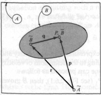
Figure 2.8.1

Hence,

{\begin{array}{l}{^{A}\mathbf{v}^{P}\ =\ {\cfrac{A}{\displaystyle d\mathbf{r}}}+{\cfrac{A_{\mathbf{\ddot{q}}}}{d t}}}\\ {\ \qquad=\ ^{A}\mathbf{v}^{\widetilde{B}}+{\cfrac{^{B}d\mathbf{q}}{d t}}+{^{A}\mathbf{o}^{B}}\ \times\ \mathbf{q}}\\ {\ \qquad=\ ^{A}\mathbf{v}^{\widetilde{B}}+{^{B}\mathbf{v}^{P}}+{^{A}\mathbf{o}^{B}}\ \times\ \mathbf{q}}\end{array}}

\widetilde{B} mayalwaysbetaken as B thatis,asthepoint of B thatcoincideswith P at the instantunderconsideration.Inthatevent,

A_{\mathbf{v}}{}^{\tilde{B}}=\sigma_{\mathbf{v}}{}^{\overline{{B}}}\qquad\mathbf{q}=0

and substitution from Eqs.(8) into Eq.(7) leads to Eq.(1).

Referring to Eq.(2.6.2),one can write

\begin{array}{l}{{\displaystyle{A_{\mathbf{a}}P=\frac{\cdots a^{-\ddots}\mathbf{v}^{\dagger}}{d t}}\ ~}}\\ {{\displaystyle{B_{\mathbf{a}}P=\frac{B_{d}B_{\mathbf{v}}P}{d t}}\ ~}}\\ {{\displaystyle{A_{\mathbf{a}}\tilde{B}=\frac{A_{d}A_{\mathbf{v}}\tilde{B}}{d t}}}}\end{array}

Substitution fromEq.（7)into Eq.(9)yields

{\begin{array}{r l}{{A_{\mathbf{{a}}}}^{P}={\frac{A{d^{A}}{\mathbf{v}}^{\bar{B}}}{d t}}+{\frac{A{d^{B}}{\mathbf{v}}^{P}}{d t}}+{\frac{A{d^{A}}{\mathbf{{0}}^{B}}}{d t}}\times\mathbf{{q}}+{\mathbf{{}}^{A}}{\mathbf{{0}}^{B}}\times{\frac{A{d}{\mathbf{q}}}{d t}}}\\ {={A_{\mathbf{{a}}}}^{\tilde{\mathbf{{a}}}}+{\frac{B{d^{B}}{\mathbf{v}}^{P}}{d t}}+{\mathbf{{}}^{A}}{\mathbf{{0}}^{B}}\times{\mathbf{{}}^{B}}{\mathbf{{v}}}^{P}+{\mathbf{{}}^{A}}{\mathbf{{\bar{q}}}}^{B}\times\mathbf{{q}}}\\ {+\mathbf{{\}}^{A}{\mathbf{{0}}}^{B}\times\left({\frac{B{d}{\mathbf{q}}}{d t}}+{\mathbf{{}}^{A}}{\mathbf{{0}}^{B}}\times\mathbf{{q}}\right)}\\ {(2.3.1)\qquad\qquad\qquad\qquad\qquad\qquad\qquad\qquad\qquad\qquad{\left({2.5}\right)}\end{array}}

and, if \pmb{\widetilde{B}} is once again taken as \pmb{\overline{{B}}}. this reduces to

{}^{A}{\pmb a}^{P}\;=\;{}^{A}{\pmb a}^{\bar{B}}\;+\;{}^{B}{\pmb a}^{P}\,+\,{}^{A}{\pmb\omega}^{B}\,\times\,{}^{B}{\mathbf v}^{P}\,+\,{}^{A}{\mathbf\omega}^{B}\,\times\,{}^{B}{\mathbf v}^{P}

in agreement with Eq. (2).

Example In the examples in Secs. 2.6 and 2.7, expressions for the velocity and the accelerationof \boldsymbol{P}_{1} in \pmb{A} were found by appealing to the definitions of velocity and acceleration, respectively. Alternatively, one can proceed as follows.

If \bar{\pmb{B}} is the point of \pmb{B} that coincides with \boldsymbol{P}_{1} (see Fig. 2.6.1), then \bar{\pmb{B}} moves on a circle of radius \pmb q_{1} , and

{\pmb{\mathfrak{s}}}{\pmb{\bar{s}}}=-\omega{\pmb q}_{1}{\pmb b}_{z}

while (remember that \omega is a constant)

{}^{A}\!{\mathfrak{a}}^{B}=\,-\omega^{2}q_{1}{\mathfrak{b}}_{x}

The velocity and acceleration of \boldsymbol{P}_{1} in \pmb{B} are

{\pmb{{\cal B}}}_{{\bf v}}P_{1}=\dot{q}_{1}{\bf b}_{x}+\dot{q}_{2}{\bf b}_{y}

and

{\displaystyle{\cal B}_{\bf a}{\cal P}_{1}=\ddot{q}_{1}{\bf b}_{x}+\ddot{q}_{2}{\bf b}_{y}}

respectively, and the angular velocity of \pmb{B} in \pmb{A} is given by

\begin{array}{c}{{A_{\mathbf{0}}B}}\\ {{(2.2.1)}}\end{array}\!\!\!\omega\mathbf{b}_{y}

Thus,

{\bf\nabla}^{A}{\bf v}^{P_{1}}={\bf\nabla}\!-\!\omega q_{1}{\bf b}_{z}+\dot{q}_{1}{\bf b}_{x}\;+\;\dot{q}_{2}\,{\bf b}_{y}

in agreement with Eq. (2.6.7), and

{\bf\Gamma}^{A}{\bf a}^{P_{1}}=\mathrm{~-}\omega^{2}q_{1}{\bf b}_{x}+\,\ddot{q}_{1}{\bf b}_{x}\,+\,\ddot{q}_{2}\,{\bf b}_{y}-\,2\omega\dot{q}_{1}{\bf b}_{z}

which is the result previously recorded as Eq. (2.7.5)

2.9 CONFIGURATION CONSTRAINTS

The configuration of a set S of \pmb{\nu} particles P_{1},...,P_{\nu} in a reference frame A is known whenever the position vector of each particle relative to a point fixed in A is known. Thus, v vector quantities, or, equivalently, \mathbf{3}\upnu scalar quantities, are required for the specification of the configuration of S in \pmb{A}

If the motion of \boldsymbol{s} is affected by the presence of bodies that come into contact with one or more of P_{1},...,P_{\nu} , restrictions are imposed on the positions that the affected particles may occupy, and \pmb{s} is said to be subject to configuration constraints;

an equation expressing such a restriction is called a holonomic constraint equation.If \mathbf{a}_{x} \mathbf{a}_{y} ， {\mathfrak{a}}_{z} are mutually perpendicular unit vectors fixed in A and x_{i},y_{i},z_{i}, called Cartesian coordinates of P_{i} in A , are defined as

x_{i}\triangleq\mathbf{p}_{i}\cdot\mathbf{a}_{x}\qquad y_{i}\triangleq\mathbf{p}_{i}\cdot\mathbf{a}_{y}\qquad z_{i}\triangleq\mathbf{p}_{i}\cdot\mathbf{a}_{z}\qquad(i=1,\ldots,\nu)

where \mathbf{p}_{i} is the position vector from a point \upsilon fixed in A to the point P_{i} then a holonomic constraint equation has the form

f(x_{1},y_{1},z_{1},\dots,x_{v},y_{v},z_{v},t)=0

where t is the time. Holonomic constraint equations are classified as rheonomic or scleronomic, according to whether the function f does, or does not, contain t explicitly.

Example Figure2.9.1showstwosmall blocks, P_{1} and P_{2} ,connected by a thin rod R of length L ,and constrained to remain between two parallel panes of glass that are attached to each other, forming a rigid body B_{\cdot} This body is made to rotate at a constant rate \omega about a line \boldsymbol{Y} fixed both in B and in a reference frame A Treating P_{1} and P_{2} as a set {\cal{S}} of two particles, and letting \mathbf{p}_{1} and {\bf p}_{2} be their position vectors relative to the point o shown in Fig.2.9.1, one can express \mathbf{p}_{1} and \mathbf{p}_{2} as

{\bf p}_{i}=x_{i}{\bf a}_{x}+y_{i}{\bf a}_{y}+z_{i}{\bf a}_{z}\qquad(i=1,2)

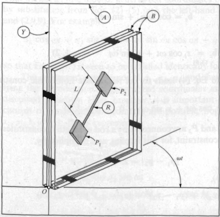
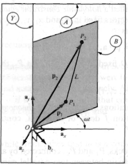
Figure 2.9.2

where \mathbf{a}_{x} ， \mathbf{a}_{y} {\bf a}_{z} aremutuallyperpendicular unitvectors fixed in A asshown inFig.2.9.2.Therequirement that \boldsymbol{P}_{1} and P_{2} remainatall timesbetweenthe twopanes ofglass isfulfilledif,and onlyif

\mathbf{p}_{i}\cdot\mathbf{b}_{z}=0\qquad(i=1,2)

where \mathfrak{b}_{z} is a unitvectornormaltotheplane determined bythepanesof glass, asindicatedinFig.2.9.2.Now,

\mathbf{b}_{z}=\cos\omega t\mathbf{a}_{z}+\sin\omega t\mathbf{a}_{x}

Hence,

p_{i}\cdot{\bf b}_{z}={\bf\nabla}_{z_{i}}\cos{\omega t}+x_{i}\sin{\omega t}\qquad(i=1,2)

andsubstitutionintoEq.（4)leadstotherheonomicholonomicconstraint equations

z_{i}\cos{\omega t}+x_{i}\sin{\omega t}=0\qquad(i=1,2)

Thefactthat P_{1} and P_{2} areconnectedbyarodof length L constitutesone moreconfigurationconstraint,forthisimplies,andisimpliedby

|\mathbf{p}_{1}-\mathbf{p}_{2}|=L

or,in view of Eqs.(3),

[(x_{1}-x_{2})^{2}+(y_{1}-y_{2})^{2}+(z_{1}-z_{2})^{2}]^{1/2}-L=0

Since in this equation,in contrast with Eq. (7), t doesnotappear explicitly, Eq.(9)is a scleronomicholonomic constraint equation.

2.10 GENERALIZED COORDINATES

When a set s of v particles P_{1},\dots,P_{v} is subject to constraints (see Sec.2.9) represented by M holonomic constraint equations, only

\boldsymbol{n}\triangleq\boldsymbol{3}\nu-\boldsymbol{M}

of the 3v Cartesian coordinates x_{i},y_{i},z_{i}\,(i=1,\ldots,\nu) of S in a reference frame \pmb{A} are independent of each other. Under these circumstances one can express each of x_{i},y_{i},z_{i}\,(i=1,\ldots,\nu) as a single-valued function of the time t and \pmb{n} functions of t say, q_{1}(t),\ldots,q_{n}(t), in such a way that the constraint equations are satisfied identically for all values of t and q_{1},\ldots,q_{n} in a given domain. The quantities q_{1},\ldots,q_{n} are called generalized coordinates for s in \pmb{A}

Example For the set s in the example in Sec. 2.9, \nu=2 and M=3. Hence n=3 . Three generalized coordinates for s in \pmb{A} may be introduced by expressing x_{i},y_{i},z_{i}\,(i=1,2) as

\begin{array}{l}{{x_{1}=q_{1}\cos{\omega t}\qquad y_{1}=q_{2}\qquad z_{1}\,=\,-q_{1}\sin{\omega t}}}\\ {{x_{2}=(q_{1}+L\cos{q_{3}})\cos{\omega t}}}\\ {{y_{2}=q_{2}+L\sin{q_{3}}}}\\ {{z_{2}=\,-(q_{1}+L\cos{q_{3}})\sin{\omega t}}}\end{array}

That q_{1},q_{2},q_{3} are, indeed, generalized coordinates of s in \pmb{A} may be verified by substituting from Eqs. (2)-(5) into the left-hand members of Eqs. (2.9.7) and (2.9.9). For example,

z_{1}\cos\omega t+x_{1}\sin\omega t=-q_{1}\sin\omega t\cos\omega t+q_{1}\cos\omega t\sin\omega t\equiv0

so that Eq. (2.9.7) is seen to be satisfied identically for i=1

The geometric significance of q_{1},q_{2},q_{3} and, hence, the rationale underlying the introduction of generalized coordinates as in Eqs. (2)-(5), will be discussed presently. First, however, it is important to point out that other choices of generalized coordinates are possible. Suppose, for example, that x_{i},y_{i},z_{i}\,(i=1,2) are expressed as

\begin{array}{r l}&{x_{1}=q_{1}\cos q_{2}\cos\omega t}\\ &{y_{1}=q_{1}\sin q_{2}}\\ &{z_{1}=-q_{1}\cos q_{2}\sin\omega t}\\ &{x_{2}=[(q_{1}+L\cos q_{3})\cos q_{2}-L\sin q_{2}\sin q_{3}]\cos\omega t}\\ &{y_{2}=(q_{1}+L\cos q_{3})\sin q_{2}+L\cos q_{2}\sin q_{3}}\\ &{z_{2}=-[(q_{1}+L\cos q_{3})\cos q_{2}-L\sin q_{2}\sin q_{3}]\sin\omega t}\end{array}

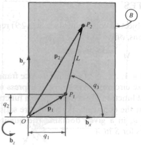
Figure 2.10.1

Then Eqs.(2.9.7) and (2.9.9) are satisfied identically,which means that,once again, q_{1} q_{2} q_{3} are generalized coordinates of s in A

The generalized coordinates introduced inEqs.(2)-(5)may beregarded asmeasures of two distances and an angle as indicated in Fig.2.10.1.This may be seen as follows.If {\mathfrak{b}}_{x} ，by， \mathbf{b}_{z} aremutually perpendicularunit vectors directed as inFig.2.10.1,then \mathbf{p}_{1} and \Psi_{2} canbewritten

\mathbf{p}_{1}=q_{1}\mathbf{b}_{x}+q_{2}\mathbf{b}_{y}\qquad\mathbf{p}_{2}=\mathbf{p}_{1}+L\cos q_{3}\mathbf{b}_{x}+L\sin q_{3}\mathbf{b}_{y}

and

x_{1}\triangleq\mathbf{\Gamma}\,\mathbf{p}_{1}\cdot\mathbf{a}_{x}=q_{1}\mathbf{b}_{x}\cdot\mathbf{a}_{x}+q_{2}\mathbf{b}_{y}\cdot\mathbf{a}_{x}

y_{1}\triangleq\!\!\begin{array}{r}{\mathbf{p}_{1}\cdot\mathbf{a}_{y}=q_{1}\mathbf{b}_{x}\cdot\mathbf{a}_{y}+q_{2}\mathbf{b}_{y}\cdot\mathbf{a}_{y}}\end{array}

z_{1}\triangleq\underset{(2,9,1)}{\b{\mathbf{p}}}_{1}\cdot\pmb{\mathscr{s}}_{\iota}=\underset{(13)}{\,\boldsymbol{q}}_{1}\pmb{\mathbf{b}}_{\iota}\cdot\pmb{\mathbf{a}}_{\iota}+q_{2}\,\pmb{\mathfrak{b}}_{\iota}\cdot\pmb{\mathbf{a}}_{\iota}

The dot-products appearing in these equations are evaluated most conveniently by referring toTable 2.10.1,which is a concise way of stating the sixequationsthatrelate \mathbf{a}_{x},\mathbf{a}_{y},\mathbf{a}_{z} to \mathbf{b}_{x},\mathbf{b}_{y},\mathbf{b}_{z}. Thus onefindsthatEqs.(14)-(16) givewaytopreciselyEqs.(2).

Table2.10.1

<html>

	bx by b.
ax ay a,	0 sinot 0 1 0 sin cot 0 coswt

</html>

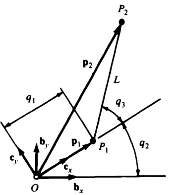
Figure 2.10.2

Similarly,

\begin{array}{r l}&{x_{2}\quad\triangleq\quad\pmb{\mathrm{p}}_{2}\cdot\mathbf{a}_{x}\,=\,\pmb{\mathrm{p}}_{1}\cdot\mathbf{a}_{x}+L\cos q_{3}\,\pmb{\mathrm{b}}_{x}\cdot\mathbf{a}_{x}+L\sin q_{3}\,\pmb{\mathrm{b}}_{y}\cdot\mathbf{a}_{x}}\\ &{\qquad\qquad\qquad\qquad\qquad\qquad=q_{1}\cos\omega t\,+\,L\cos q_{3}\cos\omega t}\\ &{\qquad\qquad\qquad\qquad\qquad\qquad\qquad\qquad\qquad(14.\,\mathbf{Table}\,2.10.1)}\end{array}

which is the same as Eq. (3), and when y_{2} and z_{2} are formed correspondingly, Eqs. (4) and (5) are recovered.

In the case of the generalized coordinates appearing in Eqs. (7)-(12), \pmb q_{1} may be interpreted as the distance from o to P_{1} , and \boldsymbol{q}_{2} and \boldsymbol{q}_{3} as the angles indicated in Fig. 2.10.2. To see this, express \pmb{{\mathsf{p}}}_{1} and \pmb{{\mathbb P}}_{2} as

\begin{array}{r}{{\bf p}_{1}=q_{1}{\bf c}_{x}\qquad{\bf p}_{2}={\bf p}_{1}+L\cos q_{3}{\bf c}_{x}+L\sin q_{3}{\bf c}_{y}\,}\end{array}

where \mathfrak{c}_{x} and \mathbf{c_{y}} are the unit vectors shown in Fig. 2.10.2, and form x_{i},\,y_{i} z_{i}\,(i=1,2) in accordance with Eqs. (2.9.1).

2.11 NUMBER OF GENERALIZED COORDINATES

The number n of generalized coordinates of a set S of \pmb{\nu} particles in a reference frame \pmb{A} (see Sec.2.10) is the smallest number of scalar quantities such that to every assignment of values to these quantities and the time t (within a domain of interest) there corresponds a definite admissible configuration of s in \pmb{A} . Frequently, one can find \pmb{n} by inspection rather than by determining the number M of holonomic constraint equations (see Sec. 2.9) and then subtracting M from \,\mathfrak{z}_{v} For example, suppose that S consists of \upnu particles P_{1},...,P_{\nu} forming a rigid body \pmb{B} that is free to move in A. Then there corresponds a definite admissible configuration of Sin \pmb{A} to every assignment of values to three Cartesian coordinates o one particle of \pmb{B} and three angles that characterize the orientation of \pmb{B} in \pmb{A} Hence, \pmb{n}=6. The same conclusion is obtained formally by letting \mathfrak{p}_{1},\ldots,\mathfrak{p}_{\nu} be the position vectors from a point fixed in \pmb{A} to P_{1},...,P_{\nu} , respectively, and noting that rigidity can be ensured by letting P_{1},P_{2} , and \boldsymbol{P_{3}} be noncollinear particles and requiring (1) that the distances between \boldsymbol{P}_{1} and P_{2},P_{2} and \boldsymbol{P_{3}} , and \boldsymbol{P_{3}} and \boldsymbol{P}_{1} remain constant, so that

\begin{array}{c}{{({\bf p}_{1}\mathrm{~-~}{\bf p}_{2})^{2}=c_{1}}}\\ {{\ }}\\ {{({\bf p}_{2}\mathrm{~-~}{\bf p}_{3})^{2}=c_{2}}}\\ {{\ }}\\ {{({\bf p}_{3}\mathrm{~-~}{\bf p}_{1})^{2}=c_{3}}}\end{array}

where c_{1},\,c_{2},\,c_{3} are constants, and (2) that the distances between each of the remaining v-3 particles and each of P_{1},P_{2} ,and \boldsymbol{P_{3}} remain constant, that is,

\begin{array}{r l}{({\bf p}_{i}-{\bf p}_{1})^{2}=c_{i1}\quad}&{{}(i=4,\ldots,\nu)}\\ {({\bf p}_{i}-{\bf p}_{2})^{2}=c_{i2}\quad}&{{}(i=4,\ldots,\nu)}\\ {({\bf p}_{i}-{\bf p}_{3})^{2}=c_{i3}\quad}&{{}(i=4,\ldots,\nu)}\end{array}

where c_{i j}\:(i=4,\ldots,\nu;j=1,2,3) are constants. The number M of holonomic constraint equations is thus given by

M=3+3(\nu-3)=3\nu-6

and it follows that

\begin{array}{r}{n\ \ =\ \ 3\nu\,-\,M=3\nu-(3\nu-6)=6}\\ {(2.10.1)}\end{array}

2.12 GENERALIZED SPEEDS

As will be seen presently, expressions for angular velocities of rigid bodies and velocities of points of a system S whose configuration in a reference frame \pmb{A} is characterized by \pmb{n} generalized coordinates q_{1},\ldots,q_{n} (see Sec. 2.10) can be brought into particularly advantageous forms through the introduction of \pmb{n} quantities u_{1},\ldots,u_{n} ,called generalized speeds for s in \pmb{A} , these being quantities defined by equations of the form

u_{r}\triangleq\sum_{s\,=\,1}^{n}\,Y_{r s}{\dot{q}}_{s}+Z_{r}\,\qquad(r=1,\dots,n)

where Y_{r s} and Z_{\nu} are functions of q_{1},\ldots,q_{n} , and the time t. These functions must be chosen such that Eqs. (1) can be solved uniquely for {\dot{q}}_{1},\dots,{\dot{q}}_{n} . Equations (1) are called kinematical differential equations for \boldsymbol{s} in \pmb{A}

Example Letting \boldsymbol{s} be the set of two particles considered in the example in Sec. 2.9, and using as generalized coordinates the quantities q_{1},q_{2},q_{3} indicated in Fig. 2.10.1, one may define three generalized speeds as

u_{1}\triangleq\dot{q}_{1}\cos{\omega t}-\omega q_{1}\sin{\omega t}\qquad u_{2}\triangleq\dot{q}_{2}\qquad u_{3}\triangleq\dot{q}_{3}

In that event, the functions \pmb{Y_{r s}} and {\bf Z}_{\mathrm{{r}}} (r,s=1,2,3 ) of Eq. (1) are

\begin{array}{r l r l r l}&{Y_{11}=\cos{\omega t}}&{Y_{12}=Y_{13}=0}&&{Z_{1}=-\omega q_{1}\sin{\omega t}}\\ &{Y_{21}=\quad0}&&{Y_{22}=1}&&{Y_{23}=0}&&{Z_{2}=0}\\ &{Y_{31}=\quad0}&&{Y_{32}=0}&&{Y_{33}=1}&&{Z_{3}=0}\end{array}

and, solved for {\dot{q}}_{1},{\dot{q}}_{2},{\dot{q}}_{3} , Eqs. (2) yield

\dot{q}_{1}=u_{1}\;\mathrm{sec}\;\omega t\,+\,\omega q_{1}\;\mathrm{tan}\;\omega t\qquad\dot{q}_{2}=u_{2}\qquad\dot{q}_{3}=u_{3}

Since sec wt and tan wt become infinite whenever wt is equal to an odd multiple of \scriptstyle\pi/2 rad, Eqs. (2) furnish acceptable definitions of u_{1},u_{2},u_{3} exceptwhen ot takes on one of these values.

As an alternative to Eqs. (2), one might let

u_{1}\,\triangleq\,\dot{q}_{1}\mathtt{c}_{3}\,+\,\dot{q}_{2}\mathtt{s}_{3}\qquad u_{2}\,\triangleq\,-\dot{q}_{1}\mathtt{s}_{3}\,+\,\dot{q}_{2}\mathtt{c}_{3}\qquad u_{3}\triangleq\,\dot{q}_{3}

where {\mathfrak{s}}_{3} and \mathsf{c}_{3} stand for sin \boldsymbol{q}_{3} and cos \pmb q_{3} , respectively. Then Z_{r}=0\;(r= 1, 2, 3), and {\dot{q}}_{1},{\dot{q}}_{2},{\dot{q}}_{3} are given by

\dot{q}_{1}=u_{1}\mathsf{c}_{3}-u_{2}\mathsf{s}_{3}\qquad\dot{q}_{2}=u_{1}\mathsf{s}_{3}+u_{2}\mathsf{c}_{3}\qquad\dot{q}_{3}=u_{3}

Here, no value of wot needs to be excluded. Finally, suppose that u_{1},u_{2},u_{3} are defined as

u_{1}\triangleq\dot{q}_{1}\qquad u_{2}\triangleq\dot{q}_{2}\qquad u_{3}\triangleq\dot{q}_{3}

While these definitions of u_{1},\,u_{2},\,u_{3} are simpler than those in Eqs. (2) and Eqs. (7), the latter are preferable in certain contexts, as will presently become apparent.

The motivation for introducing u_{1},u_{2} , and {\pmb u}_{3} as in Eqs. (2), (7), and (9) is the following. The velocity of P_{1} in \pmb{A} can be expressed in a variety of ways, such as

\begin{array}{r l}&{^{A}\mathbf{v}^{P_{1}}\quad=\quad\dot{q}_{1}\mathbf{b}_{x}+\dot{q}_{2}\mathbf{b}_{y}-\omega q_{1}\mathbf{b}_{z}}\\ &{\qquad\quad(2.6.7)}\\ &{\qquad\quad=\quad(\dot{q}_{1}\mathrm{c}_{3}+\dot{q}_{2}\mathrm{s}_{3})\mathbf{e}_{x}+(-\dot{q}_{1}s_{3}+\dot{q}_{2}\mathrm{c}_{3})\mathbf{e}_{y}-\omega q_{1}\mathbf{e}_{z}}\\ &{\qquad\quad(2.6.8)}\end{array}

and (see Fig. 2.9.2 for \mathbf{a}_{x},\mathbf{a}_{y},\mathbf{a}_{z})

\begin{array}{r}{{^A\!\mathbf{v}^{P_{1}}}=(\dot{q}_{1}\cos\omega t-\omega q_{1}\sin\omega t)\mathbf{a}_{x}+\dot{q}_{2}\mathbf{a}_{y}-(\dot{q}_{1}\sin\omega t+\omega q_{1}\cos\omega t)\mathbf{a}_{z}}\end{array}

When Eqs. (9) are used to define {\pmb u}_{1},{\pmb u}_{2} , and \pmb{u}_{3} , Eq. (10) can be rewritten as

{\pmb{{A}}}_{{\bf{v}}}{\pmb{{P}}}_{1}=u_{1}{\pmb{{b}}}_{x}+u_{2}{\pmb{{b}}}_{y}-\omega q_{1}{\pmb{{b}}}_{z}

Similarly, the definitions of {\pmb u}_{1},{\pmb u}_{2} and \pmb{u}_{3} in accordance with Eqs. (7) permit one to replace Eq. (11) with a relationship having the same simple form as Eq. (13), namely,

^{A}\mathbf{v}^{P_{1}}=u_{1}\mathbf{e}_{x}+u_{2}\mathbf{e}_{y}-\omega q_{1}\mathbf{e}_{z}

Finally, with the aid of Eqs. (2), (6), and (12), one obtains

A_{\mathbf{\bar{v}}}P_{1}=u_{1}\mathbf{a}_{x}+u_{2}\mathbf{a}_{y}-(u_{1}\tan\omega t+\omega q_{1}\sec\omega t)\mathbf{a}_{z}

Here, the third component is a bit more complicated than in Eqs. (13) and (14), but the introduction of generalized speeds has led to a noticeable simplification, nevertheless. The guiding idea in writing Eqs. (7) and (2) was thus to enable one to replace Eqs. (11) and (12), respectively, with expressins having, as nearly as possible, the same simple form as Eq. (10). As for Eq<. (9), their use does not lead to any simplifications since Eq. (10) cannot be simplified further, but they were included to show that the concept of generalized speeds remains applicable even under these circumstances.

The simplification of an angular velocity expression through the use of generalized speeds can be illustrated by returning to the example in Sec. 2.4. The angular velocity expression recorded in Eq. (2.4.10), while simple in form, is unsuitable for certain purposes because \mathbf{k}_{2},\,\mathbf{k}_{7} ,and {\bf k}_{3} are not mutually perpendicular. To overcome this difficulty, one can let \bf{k_{4}} be a unit vector directed as shown in Fig. 2.4.1 and note that {\bf k}_{3} then is given by

{\bf k}_{3}=\mathrm{-}(\cos{q_{2}}\,{\bf k}_{2}+\sin{q_{2}}\,{\bf k}_{4})

so that Eq. (2.4.10) may be replaced with

\begin{array}{r}{\mathbf{\Gamma}^{A}\!\!\mathbf{o}^{B}=\dot{q}_{1}\mathbf{k}_{2}+\dot{q}_{2}\mathbf{k}_{7}-\dot{q}_{3}(\cos q_{2}\mathbf{k}_{2}+\sin q_{2}\mathbf{k}_{4})}\\ {=(\dot{q}_{1}-\dot{q}_{3}\cos q_{2})\mathbf{k}_{2}+\dot{q}_{2}\mathbf{k}_{7}-\dot{q}_{3}\sin q_{2}\mathbf{k}_{4}}\end{array}

which reduces to

^{A}{\bf{\omega}}{}^{B}=u_{1}{\bf{k}}_{2}+u_{2}\,{\bf{k}}_{7}+u_{3}\,{\bf{k}}_{4}

if generalized speeds u_{1},u_{2} , and \pmb{u}_{3} are defined as

u_{1}\,\triangleq\,\dot{q}_{1}\,-\,\dot{q}_{3}\,\cos\,q_{2}\qquad u_{2}\,\triangleq\,\dot{q}_{2}\qquad u_{3}\,\triangleq\,-\,\dot{q}_{3}\,\sin\,q_{2}

While generalized speeds can be time-derivatives of a function of the generalized coordinates and the time t [for example, u_{1},u_{2} , and \pmb{u}_{3} as defined in Eqs. (2) are, respectively, the time-derivatives of \pmb q_{1} cos wt, \pmb q_{2} , and q_{3}] this is not always the case. Consider, for instance, \pmb{u}_{1} as defined in Eq. (7), and assume the existence of a function f\,\mathrm{of}\,q_{1},q_{2},q_{3} , and t such that

\frac{d f}{d t}=u_{1}

for all values of q_{1},q_{2},q_{3} , and t in some domain of these variables. Then

\begin{array}{c}{{\displaystyle{\frac{d f}{d t}}_{(1.9.3)}=\,{\frac{\partial f}{\partial q_{1}}}\,{\dot{q}}_{1}\,+\,{\frac{\partial f}{\partial q_{2}}}\,{\dot{q}}_{2}\,+\,{\frac{\partial f}{\partial q_{3}}}\,{\dot{q}}_{3}\,+\,{\frac{\partial f}{\partial t}}}}\\ {{\mathrm{~\boldmath~\mu~}_{=~}}}\\ {{\displaystyle{\dot{q}}_{1}{\dot{\bf c}}_{3}\,+\,{\dot{q}}_{2}\,{\mathsf{s}}_{3}}}\end{array}

which imples that

\frac{\partial f}{\partial q_{1}}=\mathrm{c}_{3}\qquad\frac{\partial f}{\partial q_{2}}=\mathrm{s}_{3}\qquad\frac{\partial f}{\partial q_{3}}=0\qquad\frac{\partial f}{\partial t}=0

The first and third of these equations are incompatible with each other, for they lead to different expressions for \partial^{2}f/\partial q_{1}\partial q_{3} . Thus, the hypothesis that f exists such that Eq. (20) is satisfied is untenable.

2.13 MOTION CONSTRAINTS

It can occur that, for physical reasons, the generalized speeds u_{1},\ldots,u_{n} for a system S in a reference frame A (see Sec. 2.4) are not independent of each other. In that event, s is said to be subject to motion constraints, and an equation that relates u_{1},\ldots,u_{n} to each other is called a nonholonomic constraint equation.

When a system S is not subject to motion constraints, then s is said to be a holonomic system possessing n degrees of freedom in \pmb{A} .If s is subject to motion constraints, s is called a nonholonomic system.

When all nonholonomic constraint equations can be expressed as the m relationships

u_{r}=\sum_{s\,=\,1}^{p}\,A_{r s}u_{s}+B_{r}\,\,\,\,\,\,\,\,\,\,\,\,(r=p\,+\,1,\ldots,n)

where

p\triangleq n-m

and where A_{r s} and B, are functions of q_{1},\ldots,q_{n} , and the time t,s is referred to as a simple nonholonomic system possessing \pmb{p} degrees of freedom in \pmb{A}

Example The particles \boldsymbol{P}_{1} and \boldsymbol{P}_{2} considered in the example in Sec. 2.9 form a holonomic system possessing three degrees of freedom in \pmb{A} . Suppose that \boldsymbol{P}_{2} is replaced with a small sharp-edged circular disk \pmb{D} whose axis is normal to the rod \pmb R and parallel to the plane in which \pmb R moves, as indicated in Fig. 2.13.1; further, that \pmb{D} comes into contact with the two panes of glass at the points D_{1} and D_{2} . Then it may be assumed that D^{*} , the center of \pmb{D} , can move freely in \pmb{B} in the direction of \pmb R , but is prevented from moving perpendicularly to \pmb R a condition that may be stated analytically in terms of \pmb{{\cal B}}_{\mathbf{v}}\pmb{{\cal D}}^{\star} , the velocity of D^{\ast} in \pmb{B} as

\begin{array}{l}{{{\cal B}_{\Psi}{\cal D}^{\star}\cdot\mathbf{e}_{y}=0}}\\ {{\ }}\\ {{{\cal B}_{\Psi}{\cal D}^{\star}\cdot\mathbf{e}_{z}=0}}\end{array}

where \mathbf{e_{y}} and \mathbf{e}_{z} are unit vectors directed as shown in Fig. 2.13.1. Now,

\begin{array}{r l r}{B_{\mathbf{V}}D^{\star}}&{{}=}&{{\cal A}_{\mathbf{V}}D^{\star}\,-\,{\cal A}_{\mathbf{V}}\tilde{\cal B}}\end{array}

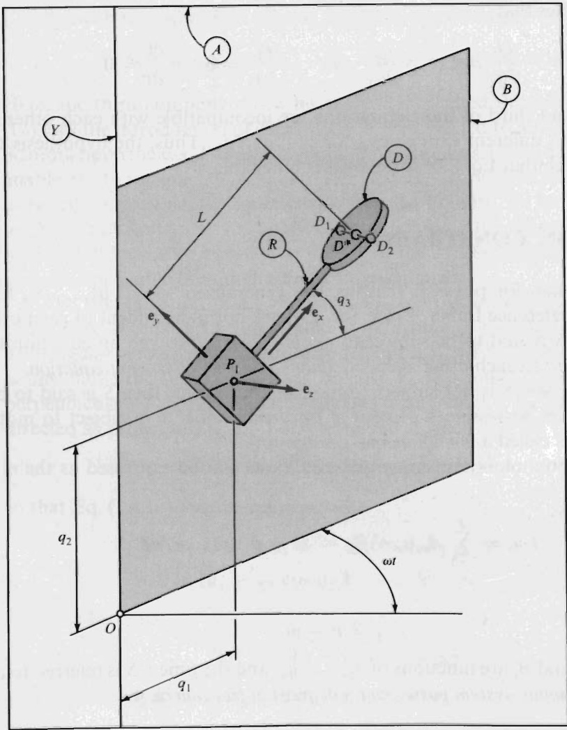
Figure 2.13.1

where \bar{B} is the point of B withwhich D^{*} coincides. This point moves on a circle ofradius q_{1}+L{\mathsf{c}}_{3} andhas thevelocity

^{A}\mathbf{v}^{\bar{B}}=\mathbf{\varepsilon}-\omega(q_{1}+L\mathbf{c}_{3})\mathbf{e}_{z}

Asfor {}^{A}\mathbf{v}^{D^{\ast}} this is precisely the velocity of P_{2} in the example in Sec. 2.6, and is, therefore,given by

{{\bf{\cal A}}_{\bf{V}}}^{D^{\bf{\dagger}}}{}_{({\bf{\bar{\alpha}}},{\bf{\bar{\alpha}}})3}^{}({\dot{q}}_{1}{\bf{c}}_{3}+{\dot{q}}_{2}{\bf{s}}_{3}){\bf e}_{x}+(-{\dot{q}}_{1}{\bf{s}}_{3}+{\dot{q}}_{2}{\bf{c}}_{3}+{\cal L}{\dot{q}}_{3}){\bf e}_{y}-\omega(q_{1}+{\cal L}{\bf c}_{3}){\bf e}_{z}

Hence,

{\bf\nabla}^{B}{\bf v}^{D^{\star}}={\bf\nabla}(\dot{q}_{1}{\bf c}_{3}+\dot{q}_{2}{\bf s}_{3}){\bf e}_{x}+(-\dot{q}_{1}{\bf s}_{3}+\dot{q}_{2}{\bf c}_{3}+L\dot{q}_{3}){\bf e}_{y}

and Eq. (3) leads to

-{\dot{q}}_{1}s_{3}+{\dot{q}}_{2}{\sf c}_{3}+L{\dot{q}}_{3}\mathop{=}_{\dots}0

while Eq. (4) is satisfied identically. Furthermore, if generalized speeds u_{1},u_{2} and \pmb{u}_{3} are introduced as in Eqs. (2.12.2), so that Eqs. (2.12.6) apply, then Eq. (9) gives rise to the nonholonomic constraint equation

u_{3}=\frac{1}{L}[(u_{1}\;\mathrm{sec}\;\omega t+\omega q_{1}\;\mathrm{tan}\;\omega t)\mathrm{s}_{3}-u_{2}\,\mathrm{c}_{3}]

Thus, m=1 p=n-m=3-1=2, and \boldsymbol{P}_{1} and \pmb{D} are seen to form a simple nonholonomic system possessing two degrees of freedom in \pmb{A} . The functions A_{r s} and B_{r}\,(r=3;s=1,2) of Eq. (1) are

A_{31}={\frac{s_{3}}{L}}\mathrm{sec}\;\omega t\qquad A_{32}={\frac{-\,c_{3}}{L}}\qquad B_{3}={\frac{s_{3}}{L}}\omega q_{1}\;\mathrm{tan}\;\omega t

If Eqs. (2.12.7), rather than Eqs. (2.12.2), are used to define u_{1},u_{2} , and \pmb{u}_{3} then Eq. (10) gives way to the much simpler relationship

u_{3}=\frac{-u_{2}}{L}

and if u_{1},u_{2} ,and \pmb{u}_{3} are defined as in Eqs. (2.12.9), the nonholonomic constraint equation is

u_{3}\ =\frac{1}{L}(u_{1}s_{3}\,-\,u_{2}{\sf c}_{3})

Before leaving this example, it is worth noting that Eq. (9) is nonintegrable ; that is, there exists no function f(q_{1},q_{2},q_{3}) which is constant throughout every time interval in which Eq. (9) is satisfied. If such a function existed, then q_{1},\,q_{2} ,and q_{3} would not be independent of each other, and thus would not be generalized coordinates.

2.14 PARTIAL ANGULAR VELOCITIES, PARTIAL VELOCITIES

If q_{1},\ldots,q_{n} and u_{1},\ldots,u_{n} are, respectively, generalized coordinates (see Sec. 2.10) and generalized speeds (see Sec. 2.12) for a simple nonholonomic system s possessing \pmb{p} degrees of freedom in a reference frame \pmb{A} , then \mathbf{\delta}_{\mathbf{\delta}}^{\mathbf{\delta}} , the angular velocity in A of a rigid body \pmb{B} belonging to S, and \mathbf{y}_{.} the velocity in A of a particle P belonging to \boldsymbol{s} canbe expressed uniquely as

\mathbf{\omega}\mathbf{\omega}\mathbf{\omega}\mathbf{\omega}\mathbf{\omega}\mathbf{\leq}\sum_{r\,=\,1}^{n}\mathbf{\omega}\mathbf{\omega}\mathbf{\omega}_{r}u_{r}\,+\,\mathbf{\omega}\mathbf{\omega}_{\!{r}}

and

{\mathbf{v}}=\sum_{r=1}^{n}{\mathbf{v}}_{r}u_{r}+{\mathbf{v}}_{t}

where \omega_{r},\,\mathbf{v}_{r}\,(r=1,\ldots,n), \mathbf{\varrho}_{t} , and \mathbf{v}_{t} are functions of q_{1},\ldots,q_{n} , and the time t The vector \mathbf{\omega}_{r} is called the rth holonomic partial angular velocity of \pmb{B} in \pmb{A} , and \mathbf{v}_{r} is referred to as the rth holonomic partial velocity of P in A

The vectors \mathbf{\omega} and \mathbf{v} can also be expressed uniquely as

\mathbf{\omega}\mathbf{\omega}\mathbf{\omega}\mathbf{\omega}\mathbf{\omega}\mathbf{\omega}\mathbf{\omega}\mathbf{\omega}\mathbf{\omega}\leq\sum_{r\,=\,1}^{p}\tilde{\mathbf{\omega}}\tilde{\mathbf{\omega}}_{r}u_{r}+\tilde{\mathbf{\omega}}\tilde{\mathbf{\omega}}_{t}

and

\mathbf{v}=\sum_{r=1}^{p}\widetilde{\mathbf{v}}_{r}\boldsymbol{u}_{r}+\widetilde{\mathbf{v}}_{t}

where \tilde{\omega}_{r},\tilde{\upnu}_{r}\,(r=1,\ldots,\,p),\tilde{\upomega}_{t} and \Tilde{\mathbf{v}}_{t} are functions of q_{1},\ldots,q_{n} , and t, Thevector \tilde{\pmb{\omega}}_{r} is called the rth nonholonomic partial angular veclocity of B in A ,while \Tilde{\mathbf{v}}_{r} is known as the rth nonholonomic partial velocity of P in \pmb{A}

When speaking of partial angular velocities and/or partial velocities, one can generally omit the adjectives “holonomic" and “nonholonomic" without loss of clarity, but the tilde notation should be used to distinguish nonholonomic partial angular velocities from holonomic ones, and similarly for partial velocities. When \pmb{p}=\pmb{n} , that is, when S is a holonomic system possessing \pmb{n} degrees of freedom in \pmb{A} , then \tilde{\pmb{\omega}}_{r}=\pmb{\omega}_{r} and \tilde{\mathbf{v}}_{r}=\mathbf{v}_{r} (r=1,\ldots,n) . It is customary not to write any tildes under these circumstances.

Derivation Solution of Eqs. (2.12.1) for {\dot{q}}_{1},\dots,{\dot{q}}_{n} yields

{\dot{q}}_{s}=\sum_{r\,=\,1}^{n}\,W_{s r}u_{r}\,+\,X_{s}\qquad(s=1,\dots,n)

where W_{s r} and X_{s} are certain functions of q_{1},\ldots,q_{n} , and t. Now, if \mathbf{b}_{1},\mathbf{b}_{2},\mathbf{b}_{3} form a right-handed set of mutually perpendicular unit vectors fixed in \pmb{B}. and if {\dot{\mathbf{b}}}_{i} denotes the first time-derivative of {\bf b}_{i} in A , then

\begin{array}{r l}{{\displaystyle{\bf\dot{b}}_{i}=\sum_{\substack{(1,9.1)\,s=1}}^{n}\frac{\partial{\bf b}_{i}}{\partial q_{s}}\,{\dot{q}}_{s}+\frac{\partial{\bf b}_{i}}{\partial t}}}&{{}}\\ {{\displaystyle=}}&{{\displaystyle\sum_{s=1}^{n}\frac{\partial{\bf b}_{i}}{\partial q_{s}}\left(\sum_{r=1}^{n}W_{s r}u_{r}+X_{s}\right)+\frac{\partial{\bf b}_{i}}{\partial t}}}\\ {{\displaystyle=}}&{{\displaystyle\sum_{r=1}^{n}\sum_{s=1}^{n}\frac{\partial{\bf b}_{i}}{\partial q_{s}}\,W_{s r}u_{r}+\sum_{s=1}^{n}\frac{\partial{\bf b}_{i}}{\partial q_{s}}\,X_{s}+\frac{\partial{\bf b}_{i}}{\partial t}}}&{{}\displaystyle(i=1,2,3)}\end{array}

where all partial differentiations of {\bf b}_{i} are performed in \pmb{A} .Consequently,

{\begin{array}{r l}{{\boldsymbol{\Theta}}}&{\mathbf{\\\theta=}\ \mathbf{b}_{1}\mathbf{\dot{b}_{2}}\cdot\mathbf{b}_{3}\mathbf{\dot{\theta}=}\mathbf{b}_{2}\mathbf{\dot{b}_{3}}\cdot\mathbf{b}_{1}\mathbf{\dot{\theta}=}\mathbf{b}_{3}\mathbf{\dot{b}_{1}}\cdot\mathbf{b}_{2}}\\ {{\boldsymbol{\mathrm{\Theta}}}}&{\mathbf{\\\theta=}\ \mathbf{b}_{1}\!\left({\displaystyle\sum_{r=1}^{n}}\ \sum_{s=1}^{n}{\frac{\partial\mathbf{b}_{2}}{\partial q_{s}}}\cdot\mathbf{b}_{3}\,W_{s r}u_{r}+\ \sum_{s=1}^{n}{\frac{\partial\mathbf{b}_{2}}{\partial q_{s}}}\cdot\mathbf{b}_{3}\,X_{s}+{\frac{\partial\mathbf{b}_{2}}{\partial t}}\cdot\mathbf{b}_{3}\right)}\\ &{\mathbf{\\\\}+\ \mathbf{b}_{2}\!\left({\displaystyle\sum_{r=1}^{n}}\ \sum_{s=1}^{n}{\frac{\partial\mathbf{b}_{3}}{\partial q_{s}}}\cdot\mathbf{b}_{1}\,W_{s r}u_{r}+\ \sum_{s=1}^{n}{\frac{\partial\mathbf{b}_{3}}{\partial q_{s}}}\cdot\mathbf{b}_{1}X_{s}+{\frac{\partial\mathbf{b}_{3}}{\partial t}}\cdot\mathbf{b}_{1}\right)}\\ &{\mathbf{\\\\}+\ \mathbf{b}_{3}\!\left({\displaystyle\sum_{r=1}^{n}}\ \sum_{s=1}^{n}{\frac{\partial\mathbf{b}_{1}}{\partial q_{s}}}\cdot\mathbf{b}_{2}\,W_{s r}u_{r}+\ \sum_{s=1}^{n}{\frac{\partial\mathbf{b}_{1}}{\partial q_{s}}}\cdot\mathbf{b}_{2}\,X_{s}+{\frac{\partial\mathbf{b}_{1}}{\partial t}}\cdot\mathbf{b}_{2}\right)}\end{array}}

and, if \mathbf{\omega}_{\mathbf{r}} and \mathbf{\omega}_{\mathbf{\rho}_{t}} are defined as

\omega_{r}\triangleq\sum_{s=1}^{n}\left(\mathbf{b}_{1}\frac{\partial\mathbf{b}_{2}}{\partial q_{s}}\cdot\mathbf{b}_{3}+\mathbf{b}_{2}\frac{\partial\mathbf{b}_{3}}{\partial q_{s}}\cdot\mathbf{b}_{1}+\mathbf{b}_{3}\frac{\partial\mathbf{b}_{1}}{\partial q_{s}}\cdot\mathbf{b}_{2}\right)W_{s r}\qquad(r=1,\ldots,n)

and

\begin{array}{c}{{\displaystyle{\bf{\omega}}_{t}\triangleq\sum_{s=1}^{n}\left[\left({\bf{\hat{b}}}_{1}\,\frac{\partial{\bf{b}}_{2}}{\partial q_{s}}\cdot{\bf{b}}_{3}+{\bf{b}}_{2}\,\frac{\partial{\bf{b}}_{3}}{\partial q_{s}}\cdot{\bf{b}}_{1}+{\bf{b}}_{3}\,\frac{\partial{\bf{b}}_{1}}{\partial q_{s}}\cdot{\bf{b}}_{2}\right)X_{s}\right.}}\\ {{\displaystyle{+\left.{\bf{\hat{b}}}_{1}\,\frac{\partial{\bf{b}}_{2}}{\partial q_{s}}\cdot{\bf{b}}_{3}+{\bf{b}}_{2}\,\frac{\partial{\bf{b}}_{3}}{\partial q_{s}}\cdot{\bf{b}}_{1}+{\bf{b}}_{3}\,\frac{\partial{\bf{b}}_{1}}{\partial q_{s}}\cdot{\bf{b}}_{2}\right]}}}\end{array}

respectively, then substitution from Eqs. (8) and (9) into Eq. (7) leads directly to Eq. (1).

To establish the validity of Eq. (2), let \pmb{\mathbb{p}} be the position vector from a point fixed in \pmb{A} to \pmb{P}_{\ast} and let \dot{\pmb{\mathsf{p}}} denote the first time-derivative of \pmb{P} in \pmb{A} Then

\begin{array}{r l}{\displaystyle\Psi_{\{\;2,6,1\}}=\displaystyle\hat{\mathbf{p}}_{\{\;1,9,1\}}^{\quad\quad=\quad}\sum_{s=1}^{n}\frac{\partial\mathbf{p}}{\partial q_{s}}\,\dot{q}_{s}+\frac{\partial\mathbf{p}}{\partial t}}\\ {\displaystyle=}&{\displaystyle\sum_{s=1}^{n}\frac{\partial\mathbf{p}}{\partial q_{s}}\left(\sum_{r=1}^{n}W_{s r}u_{r}+X_{s}\right)+\frac{\partial\mathbf{p}}{\partial t}}\\ {\displaystyle=}&{\displaystyle\sum_{r=1}^{n}\sum_{s=1}^{n}\frac{\partial\mathbf{p}}{\partial q_{s}}\,W_{s r}u_{r}+\sum_{s=1}^{n}\frac{\partial\mathbf{p}}{\partial q_{s}}X_{s}+\frac{\partial\mathbf{p}}{\partial t}}\end{array}

and, after defining \mathbf{v}_{\star} and \mathbf{y}_{t} as

\begin{array}{r}{\displaystyle\Psi_{r}\triangleq\,\sum_{s\,=\,1}^{n}\frac{\partial\mathbf{p}}{\partial q_{s}}\,W_{s r}\qquad(r=1,\ldots,n)}\end{array}

and

\mathbf{v}_{t}\triangleq\sum_{s=1}^{n}{\frac{\partial\mathbf{p}}{\partial q_{s}}}\,X_{s}+{\frac{\partial\mathbf{p}}{\partial t}}

respectively, one obtains Eq. (2) by substituting from Eqs. (11) and (12) into Eq. (10).

Suppose now that \pmb{s} is subject to motion constraints such that u_{1},\ldots,u_{n} are governed by Eqs. (2.13.1) Then, afer rewriting Eq. (1) as

\mathbf{\omega}\Leftrightarrow\sum_{r\,=\,1}^{p}\,\omega_{r}u_{r}\,+\,\sum_{r\,=\,p+\,1}^{n}\,\omega_{r}u_{r}\,+\,\omega_{t}

one can use Eq. (2.13.1) to obtain

\begin{array}{r l}{\lefteqn{\mathrm{\boldmath~\Lambda~}_{(0)}^{p}=\displaystyle\sum_{(1)}^{p}\mathrm{\boldmath~{\omega}~}_{r}u_{r}+\sum_{r=p+1}^{n}\mathrm{\boldmath~\omega~}_{\varepsilon_{n}}\left(\sum_{s=1}^{p}A_{r}u_{s}+B_{r}\right)+\mathrm{\boldmath~\omega~}_{0}}}\\ &{=\displaystyle\sum_{r=1}^{p}\mathrm{\boldmath~{\omega}~}_{0}\mathrm{\boldmath~\omega~}_{r}+\sum_{s=1}^{p}\sum_{r=p+1}^{n}\mathrm{\boldmath~{\omega}~}_{0}A_{r}\,{\cal u}_{s}+\sum_{r=p+1}^{n}\mathrm{\boldmath~{\omega}~}_{0}B_{r}+\mathrm{\boldmath~{\omega}~}_{0}}\\ &{=\displaystyle\sum_{r=1}^{p}\mathrm{\boldmath~{\omega}~}_{0}\mathrm{\boldmath~{\omega}~}_{r}+\sum_{r=1}^{p}\sum_{s=p+1}^{n}\mathrm{\boldmath~{\omega}~}_{0}A_{r}\,{\cal u}_{r}+\sum_{r=p+1}^{n}\mathrm{\boldmath~{\omega}~}_{0}B_{r}+\mathrm{\boldmath~{\omega}~}_{0}}\\ &{=\displaystyle\sum_{r=1}^{p}\left(\mathrm{\boldmath~{\omega}~}_{0}+\sum_{s=p+1}^{n}\mathrm{\boldmath~{\omega}~}_{0}A_{r}\right)u_{r}+\sum_{r=p+1}^{n}\mathrm{\boldmath~{\omega}~}_{0}B_{r}+\mathrm{\boldmath~{\omega}~}_{0}}\end{array}

and, after defining {\tilde{\pmb{\omega}}}, . and \tilde{\mathbf{o}}_{t} as

\tilde{\omega}_{r}\triangleq\omega_{r}+\sum_{\substack{s\,=\,p\,+\,1}}^{n}\omega_{s}\,A_{s r}\qquad(r=1,\,.\,.\,.\,,p)

and

\tilde{\omega}_{t}\triangleq\omega_{t}+\sum_{r=p+1}^{n}\omega_{r}B_{r}

one arrives at Eq. (3) by substituting from Eqs. (15) and (16) into Eq. (14). A completely analogous derivation leads from Eq. (2) to Eq. (4), provided that \Tilde{\mathbf{v}}, and \widetilde{\mathbf{v}}_{t} aredefinedas

\tilde{\nabla}_{r}\triangleq\,\mathbf{v}_{r}+\sum_{\substack{s\,=\,p+1}}^{n}\,\mathbf{v}_{s}\,A_{s r}\qquad(r=1,\ldots,p)

and

\widetilde{\mathbf{v}}_{t}\triangleq\mathbf{v}_{t}+\sum_{r=p+1}^{n}\mathbf{v}_{r}B_{r}

As will become evident later, the use of partial angular velocities and partial velocities greatly facilitates the formulation of equations of motion. Moreover, the constructing of expressions for these quantities is a simple matter involving nothing more than the inspecting of expressions for angular velocities of rigid bodies and/or expressions for velocities of particles.

Example In the example in Sec. 2.12, three sets of generalized speeds were introduced and the corresponding expressions for the velocity of the particle \boldsymbol{P}_{1} in reference frame A (see Fig. 2.9.1) were recorded in Eqs. (2.12.13)- (2.12.15). Each of these equations has precisely the same form as Eq. (2), and inspection of the equations thus permits one to identify the associated holonomic partial velocities of \boldsymbol{P}_{1} in \pmb{A} as

\begin{array}{r l r l}&{A_{\mathbf{v}_{1}}P_{1}\quad}&{=\quad\mathbf{b}_{x}}&{A_{\mathbf{v}_{2}}P_{1}\quad}&{=\quad\mathbf{b}_{y}\quad}&{A_{\mathbf{v}_{3}}P_{1}\quad}&{=\quad0}\\ &{}&{\qquad\qquad(2.12.13)}\\ &{A_{\mathbf{v}_{1}}P_{1}\quad}&{=\quad\mathbf{e}_{x}}&{A_{\mathbf{v}_{2}}P_{1}\quad=\quad\mathbf{e}_{y}}&{A_{\mathbf{v}_{3}}P_{1}\quad=\quad0}\\ &{}&{\qquad\qquad(2.12.14)}\\ &{A_{\mathbf{v}_{1}}P_{1}\quad}&{=\quad\mathbf{a}_{x}-\tan\omega t\mathbf{a}_{z}}&{A_{\mathbf{v}_{2}}P_{1}\quad=\quad\mathbf{a}_{\mathbf{v}_{2}}\mathbf{a}_{y}}&{A_{\mathbf{v}_{3}}P_{1}\quad=\quad0}\\ &{}&{\qquad\qquad(2.12.15)}\end{array}

The angular velocity of E in \pmb{A} , introduced in the example in Sec. 2.6, can be written

\begin{array}{r}{\pmb{\omega}_{\pmb{\omega}_{\pmb{\omega}_{\pmb{\omega}_{-}}}^{E}}=\quad\omega\mathbf{s}_{3}\mathbf{e}_{x}+\omega\mathbf{c}_{3}\mathbf{e}_{y}+u_{3}\mathbf{e}_{z}}\end{array}

in all three cases because \pmb{u}_{3} was defined as \dot{q}_{3} in Eqs. (2.12.2), (2.12.7), and (2.12:9). Comparing Eq. (22) with Eq. (1), one can write down the holonomic partial angular velocities of {\pmb E} in \pmb{A}

{\bf{\Psi}}^{A}{\bf{\Theta}}_{0}{\bf{\Psi}}^{E}={\bf{\Psi}}^{A}{\bf{\Theta}}_{0}{\bf{\Psi}}^{E}={\bf{e}}_{z}

To illustrate the idea of nonholonomic partial angular velocities and nonholonomic partial velocities, we confine our attention to the generalized speeds of Eqs. (2.12.7), which means that Eqs. (20) and (23) apply, and explore the effect of the motion constraint considered in the example in Sec. 2.13, which was there shown to give rise to the nonholonomic constraint equation

u_{3}\mathop{=}_{(2,13,12)}-\frac{u_{2}}{L}

As regards the partial velocities of P_{1} in \pmb{A} ; Eq. (24) makes no difference whatsoever, for u_{3} is absent from Eq. (2.12.14),the relevant expression for A_{\mathbf{V}}P_{\mathrm{:}} In other words, the two nonholonomic partial velocities of \boldsymbol{P}_{1} in \pmb{A} (there are two because n=3. m=1, and p=n-m=3-1=2) are

\begin{array}{r}{^{A}\tilde{\mathbf{v}}_{1}\,^{P_{1}}\qquad=\qquad\mathbf{e}_{x}\qquad^{A}\tilde{\mathbf{v}}_{2}\,^{P_{1}}\qquad=\qquad\mathbf{e}_{y}\ }\\ {(2.12\,.14)\qquad\qquad\qquad\qquad\qquad(2.12.14)}\end{array}

and these are the same as their holonomic counterparts in Eqs. (20). In connection with the partial angular velocities of \pmb{E} in \pmb{A} ,however,Eq. (24) matters very much, for substitution from Eq. (24) into Eq. (22) produces

{\bf{\nabla}}^{A}{\bf{\Theta}}^{E}=\omega{\bf{s}}_{3}{\bf{e}}_{x}+\omega{\bf{c}}_{3}{\bf{e}}_{y}-\left(\frac{u_{2}}{L}\right){\bf{e}}_{z}

which has the form of Eq. (3) and permits one to identify the two nonholonomic partial angular velocities of \pmb{E} in \pmb{A} as

A_{\tilde{\pmb{\omega}}_{1}}\!\!\!\!\!^{\!}\!\!\!\!\!\!^{\!}\!\!\!\!\!\!\!\!\!\!\!\!\!\!\!\!\!\!\!\!\!\!\!\!\!\!\!\!\!\!\!\!\!\!\!\!\!\!\!\!\!\!\!\!\!\!\!\!\!\!\!\!\!\!\!\!\!\!\!\!\!\!\!\!\!\!\!\!\!\!\!\!\!\!\!\!\!\!\!\!\!\!\!\!\!\!\!\!\!\!\!\!\!\!\!\!\!\!\!\!\!\!\!\!\!\!\!\!\!\!\!\!\!\!\!\!\!\!\!\!\!\!\!\!\!\!\!\!\!\!\!\!\!\!\!\!\!\!\!\!\!\!\!\!\!\!\!\!\!\!\!\!\!\!\!\!\!\!\!\!\!\!\!\!\!\!\!\!\!\!\!\!\!\!\!\!\!\!\!\!\!\!\!\!\!\!\!\!\!\!\!\!\!\!\!\!\!\!\!\!\!\!\!\!\!\!\!\!\!\!\!\!\!\!\!\!\!\!\!\!\!\!\!\!\!\!\!\!\!\!\!\!\!\!\!\!\!\!\!\!\!\!\!\!\!\!\!\!\!\!\!\!\!\!\!\!\!\!\!\!\!\!\!\!\!\!\!\!\!\!\!\!\!\!\!\!\!\!\!\!\!\!\!\!\!\!\!\!\!\!\!\!\!\!\!\!\!\!\!\!\!\!\!\!\!\!\!\!\!\!\!\!\!\!\!\!\!\!\!\!\!\!\!\!\!\!\!\!\!\!\!\!\!\!\!\!\!\!\!\!\!\!\!\!\!\!\!\!\!\!\!\!\!\!\!\!\!\!\!\!\!\!\!\!\!\!\!\!\!\!\!\!\!\!\!\!\!\!\!\!\!\!\!\!\!\!\!\!\!\!\!\!\!\!\!\!\!\!\!\!\!\!\!\!\!\!\!\!\!\!\!\!\!\!\!\!\!\!\!\!\!\!\!\!\!\!\!\!\!\!\!\!\!\!\!\!\!\!\!\!\!\!\!\!\!\!\!\!\!\!\!\!\!\!\!\!\!\!\!\!\!\!\!\!\!\!\!\!\!\!\!\!\!\!\!\!\!\!\!\!\!\!\! 

The second of these differs noticeably from its counterpart in Eq. (23)

Finally, still working with the generalized speeds of Eqs. (2.12.7), let us examine the three holonomic and two nonholonomic partial velocities of D^{\ast} in \pmb{A} (see Fig. 2.13.1). To determine these, we refer to Eqs. (2.6.13) and (2.12.7) to express \pmb{A}_{\mathbf{v}}\pmb{D}^{\star} as

^{A}{\bf v}^{D^{*}}=u_{1}{\bf e}_{x}+(u_{2}+L u_{3}){\bf e}_{y}-\omega(q_{1}+L{\bf c}_{3}){\bf e}_{z}

and note that, when Eq. (24) is taken into account, \mathbf{\deltaA_{v}}\mathbf{{\calD}^{\star}} is given by

^A{\bf v}^{D^{\star}}=u_{1}{\bf e}_{x}-\omega(q_{1}+L{\bf c}_{3}){\bf e}_{z}

Consequently, the holonomic partial velocities of D^{\ast} in \pmb{A} are

^{A}\mathbf{v}_{1}^{\phantom{\dagger}D^{\star}}\:=\:\mathbf{e}_{x}\qquad^{A}\mathbf{v}_{2}^{\phantom{\dagger}D^{\star}}\:=\:\mathbf{e}_{y}\qquad^{A}\mathbf{v}_{3}^{\phantom{\dagger}D^{\star}}\:=\:L\mathbf{e}_{y}

while the nonholonomic partial velocities of D^{*} in \pmb{A} are

A_{\widetilde{\Psi}_{1}}{}^{D^{\star}}=\textbf{e}_{x}\qquad A_{\widetilde{\Psi}_{2}}{}^{D^{\star}}\,=\,0

2.15 ACCELERATION AND PARTIAL VELOCITIES

When q_{1},\ldots,q_{n} are generalized coordinates characterizing the configuration of a system S in a reference frame \pmb{A} (see Sec. 2.10), then \mathbf{v}^{2} , the square of the velocity in \pmb{A} of a generic particle \pmb{P} of S, may be regarded as a (scalar) function of the 2n+1 independent variables q_{1},\ldots,q_{n},\ {\dot{q}}_{1},\ldots,{\dot{q}}_{n} , and t, where \dot{\pmb q}_{r} denotes the first time-derivative of q_{r}\left(r=1,\ldots,n\right) . If generalized speeds (see Sec. 2.12) are defined as

u_{r}\triangleq{\dot{q}}_{r}\qquad(r=1,\dots,n)

and \pmb{\upnu}_{\pmb{r}} denotes the rth holonomic partial velocity of \pmb{P} in \pmb{A} (see Sec. 2.14), then \pmb{\Psi}_{r} , the acceleration a of \pmb{P} in \pmb{A} , and \mathbf{v}^{2} are related to each other as follows:

\Psi_{r}\cdot\mathbf{a}={\frac{1}{2}}\left({\frac{d}{d t}}{\frac{\partial\mathbf{v}^{2}}{\partial{\dot{q}}_{r}}}-{\frac{\partial\mathbf{v}^{2}}{\partial q_{r}}}\right)\qquad(r=1,\ldots,n)

If in accordance with Eqs. (2.12.1), generalized speeds are defined as

u_{r}\triangleq\sum_{s\,=\,1}^{n}\,Y_{r s}{\dot{q}}_{s}+Z_{r}\,\qquad(r=1,\dots,n)

where Y_{r s} and Z, are functions of q_{1},\ldots,q_{n} , and the time t_{\mathrm{-}} and \pmb{\upnu}_{\pmb{r}} denotes the associated rth holonomic partial velocity of \pmb{P} in \pmb{A} (see Sec. 2.14), then

\Psi_{r}\cdot{\bf a}=\frac{1}{2}\sum_{s=1}^{n}\left(\frac{d}{d t}\frac{\partial\Psi^{2}}{\partial{\dot{q}}_{s}}-\frac{\partial\Psi^{2}}{\partial q_{s}}\right)W_{s r}\qquad(r=1,\ldots,n)

where W_{s r} is a function of q_{1},\ldots,q_{n} and t such that solution of Eqs. (3)for {\dot{q}}_{1},\dots,{\dot{q}}_{n} yields

{\dot{q}}_{s}=\sum_{r\,=\,1}^{n}\,W_{s r}u_{r}\,+\,X_{s}\qquad(s=1,\dots,n)

Finally, when s is a simple nonholonomic system possessing \pmb{p} degrees of freedom in \pmb{A} (see Sec. 2.13), so that there exist m nonholonomic constraint equations of the form

u_{r}=\sum_{s\,=\,1}^{p}A_{r s}u_{s}+B_{r}\qquad(r=p+1,\ldots,n)

then \widetilde{\mathbf{v}}_{r}\cdot\mathbf{a}, where \Tilde{\mathbf{v}}_{r} is the rth nonholonomic partial velocity of \pmb{P} in \pmb{A} (see Sec. 2.14), can be expressed in terms of \mathbf{v}^{2} (still regarded as a function of q_{1},\ldots,q_{n} \dot{q}_{1},\ldots,\dot{q}_{n} , and t )as

\begin{array}{l}{{\widetilde{\mathbf{v}}_{r}\cdot\mathbf{a}=\displaystyle\frac{1}{2}\left(\frac{d}{d t}\frac{\partial\mathbf{v}^{2}}{\partial{\dot{q}}_{r}}-\frac{\partial\mathbf{v}^{2}}{\partial q_{r}}\right)\quad}}\\ {{\qquad\displaystyle+\ \frac{1}{2}\sum_{s=p+1}^{n}\left(\frac{d}{d t}\frac{\partial\mathbf{v}^{2}}{\partial{\dot{q}}_{s}}-\frac{\partial\mathbf{v}^{2}}{\partial q_{s}}\right)A_{s r}\qquad(r=1,\ldots,p)}}\end{array}

when u_{r} is defined as in Eqs. (1), and as

\widetilde{\mathbf{v}}_{r}\cdot\mathbf{a}=\frac{1}{2}\sum_{s=1}^{n}\left[\left(\frac{d}{d t}\frac{\partial\mathbf{v}^{2}}{\partial\dot{q}_{s}}-\frac{\partial\mathbf{v}^{2}}{\partial q_{s}}\right)\left(W_{s r}+\sum_{k=\,p+1}^{n}W_{s k}A_{k r}\right)\right]\qquad(r=1,\,\ldots,p)

when \pmb{u}_{\pmb{r}} is defined as in Eq. (3).

Equations (2),(7), and (8) play essential parts in the derivations of Lagrange equations and Passerello-Huston equations (see Problem 11.12). Additionally, Eqs. (2) can facilitate the determination of accelerations, as will be shown presently.

Derivation When \pmb{u}_{\pmb{r}} is defined as in Eqs. (1), then W_{s r} in Eqs. (2.14.5) is equal to unity for s=r and vanishes otherwise, while X_{s} vanishes for s=1,\ldots,n. Consequently, Eqs. (2.14.11) and (2.14.12) reduce to

\begin{array}{l c r}{{\displaystyle\mathbf{v}_{r}~~~=~~~\frac{\partial\mathbf{p}}{\partial q_{r}}~~}}&{{(r=1,\ldots,n)}}\\ {{\null}}&{{\null}}\\ {{\displaystyle\mathbf{v}_{t}~~~=~~~\frac{\partial\mathbf{p}}{\partial t}}}&{{\null}}\end{array}

respectively. From the first of these it follows that

{\frac{\partial\mathbf{v}_{r}}{\partial q_{s}}}={\frac{\partial}{\partial q_{s}}}\left({\frac{\partial\mathbf{p}}{\partial q_{r}}}\right)_{(1.8.3)}{\frac{\partial}{\partial q_{r}}}\left({\frac{\partial\mathbf{p}}{\partial q_{s}}}\right)_{(9)}={\frac{\partial\mathbf{v}_{s}}{\partial q_{r}}}\qquad(r,s=1,\ldots,n)

while the two together lead to

{\frac{\partial\mathbf{v}_{t}}{\partial q_{r\,(10)}}}={\frac{\partial}{\partial q_{r}}}\left({\frac{\partial\mathbf{p}}{\partial t}}\right)_{(1.8.4)}{\overline{{\partial}}}_{t}{\frac{\partial\mathbf{p}}{\partial q_{r\,(9)}}}={\frac{\partial\mathbf{v}_{r}}{\partial t}}

These relationships will be used shortly.

When v is expressed as in Eq. (2.14.2) and \pmb{u}_{\pmb{r}} is replaced with \dot{\pmb q}_{r} in accordance with Eqs. (1), one can regard v as a function of the independent variables q_{1},\ldots,q_{n} {\dot{q}}_{1},\dots,{\dot{q}}_{n} , and t , in which event

\frac{\partial\dot{q}_{s}}{\partial q_{r}}=0\qquad(r,s=1,\ldots,n)

and partial differentiation of \pmb{\mathrm{v}} with respect to \pmb q_{r} gives

\begin{array}{r l}{\lefteqn{\frac{\partial\mathbf{v}}{\partial q_{r}}=\frac{\partial}{1.14.2}\frac{\partial}{\partial q_{r}}\left(\sum_{s=1}^{n}\mathbf{v}_{s}\dot{q}_{s}+\mathbf{v}_{t}\right)}}\\ &{\qquad=\underbrace{\vphantom{\frac{1}{1.1}}\sum_{s=1}^{n}\left(\frac{\partial\mathbf{v}_{s}}{\partial q_{r}}\dot{q}_{s}+\mathbf{v}_{s}\frac{\partial\dot{q}_{s}}{\partial q_{r}}\right)}_{\mathbf{1}.7.2}+\frac{\partial\mathbf{v}_{t}}{\partial q_{r}}}\\ &{\qquad=\underbrace{\sum_{s=1}^{n}\frac{\partial\mathbf{v}_{r}}{\partial q_{s}}\dot{q}_{s}+0+\frac{\partial\mathbf{v}_{t}}{\partial q_{r}}\dot{\mathbf{\Gamma}}_{(1,9.1)}\frac{\partial\mathbf{v}_{r}}{\partial t}}_{\mathbf{1};\mathbf{1};\mathbf{1};\mathbf{\Gamma}_{(1,1)}}\qquad(r=1,\dots,n)}\end{array}

while partial differentiation with respect to {\dot{\pmb q}}, produces

\frac{\partial\mathbf{v}}{\partial\dot{q}_{r}}\mathop{=}_{(2,14.2)}\frac{\partial}{\partial\dot{q}_{r}}\left(\sum_{s=1}^{n}\mathbf{v}_{s}\dot{q}_{s}+\mathbf{v}_{t}\right)=\mathbf{v}_{r}\qquad(r=1,\ldots,n)

since \pmb{\mathrm{v}}_{\pmb{s}} and \mathbf{y}_{t} are independent of {\dot{q}}_{r} , and \partial{\dot{q}}_{s}/\partial{\dot{q}}_{i} vanishes except for s=r, in which case it is equal to unity.

To conclude the derivation of Eq. (2), we note that

{\begin{array}{r l}{{\cfrac{d}{d t}}\,(\mathbf{v}_{r}\cdot\mathbf{v})={\cfrac{d\mathbf{v}_{r}}{d t}}\cdot\mathbf{v}+\mathbf{v}_{r}\cdot{\cfrac{d\mathbf{v}}{d t}}\quad}&{}\\ {={\cfrac{\partial\mathbf{v}}{\partial q_{r}}}\cdot\mathbf{v}+\mathbf{\nabla}\mathbf{v}_{r}\cdot\mathbf{a}\quad}&{(r=1,\ldots,n)}\end{array}}

which, solved for \mathbf{v}_{\star}\cdot\mathbf{a}. yields

\displaystyle\mathbf{v}_{r}\cdot\mathbf{a}\,=\,{\frac{d}{\scriptscriptstyle{(16)}}}(\displaystyle\mathbf{v}_{r}\cdot\mathbf{v})-{\frac{\partial\mathbf{v}}{\partial q_{r}}}\cdot\mathbf{v}\qquad(r=1,\ldots,n)

\begin{array}{l}{{\displaystyle{\bf v}_{r}\cdot{\bf a}{\bf\Pi}=\frac{d}{(17)}\left(\frac{\partial{\bf v}}{\partial\dot{q}_{r}}\cdot{\bf v}\right)-\frac{\partial{\bf v}}{\partial q_{r}}\cdot{\bf v}\ ~}}\\ {{\displaystyle~~~~~~~=\frac{d}{d t}\left(\frac{1}{2}\frac{\partial{\bf v}^{2}}{\partial\dot{q}_{r}}\right)-\frac{1}{2}\frac{\partial{\bf v}^{2}}{\partial q_{r}}~~~~~(r=1,\dots,n)}}\end{array}

and this is equivalent to Eqs. (2).

To establish the validity of Eqs. (4), we begin by exploring the relationship between the partial velocities associated with generalized speeds defined as in Eqs. (1), on the one hand, and partial velocities associated with generalized speeds defined as in Eqs. (3), on the other hand. Denoting the former by \mathbf{v}_{1},\ldots,\mathbf{v}_{n} ,as heretofore,we have

\boldsymbol{\mathbf{v}}\underset{(2,14.2)}{=}\sum_{r=1}^{n}\boldsymbol{\mathbf{v}}_{r}\dot{q}_{r}+\boldsymbol{\mathbf{v}}_{t}

Hence, when u_{1},\ldots,u_{n} are defined as in Eqs. (3), so that Eqs. (5) apply, we can write

\begin{array}{r l}{\lefteqn{\begin{array}{r l}{\textsf{v}=}&{\displaystyle\sum_{(19,5)}^{n}\nabla_{r}\left(\sum_{s=1}^{n}W_{r s}u_{s}+X_{r}\right)+\Psi_{t}}\\ &{=\displaystyle\sum_{r=1}^{n}\sum_{s=1}^{n}\Psi_{s}W_{s r}u_{r}+\sum_{r=1}^{n}\Psi_{r}X_{r}+\Psi_{t}}\end{array}}}\end{array}

and now we can identify the partial velocities associated with u_{1},\ldots,u_{n} ,which we denote temporarily by \overline{{\mathbf{v}}}_{1},\hdots,\overline{{\mathbf{v}}}_{n} , as the coefficients of u_{1},\ldots,u_{n} ,respectively, in Eq. (20); that is,

\overline{{\mathbb{V}}}_{r}\triangleq\sum_{s\,=\,1}^{n}\mathbb{v}_{s}\,W_{s r}\qquad(r=1,\ldots,n)

The derivation of Eqs. (4) then can be completed by dot-multiplying Eqs. (21) with a, using Eqs. (2) to eliminate \mathbf{v}_{s}\cdot\mathbf{a}~(s=1,\ldots,n). and writing \mathbf{v}_{\star} in place of \bar{\mathsf{v}}_{r}\left(r=1,\ldots,n\right)

Lastly, to obtain Eqs. (7) and (8), dot-multiply Eqs. (2.14.17) with a, showing that

\tilde{\Psi}_{r}\cdot\mathbf{a}=\Psi_{r}\cdot\mathbf{a}\,+\,\sum_{\substack{s=\,p+1}}^{n}\Psi_{s}\cdot\mathbf{a}A_{s r}\qquad(r=1,\,.\,.\,.\,,p)

and then use Eqs. (2) in connection with Eqs. (7), and Eqs. (4) in the case of Eqs. (8),to eliminate \displaystyle\mathbf{v}_{r}\cdot\mathbf{a}\left(r=1,\ldots,p\right) and \mathbf{v}_{s}\cdot\mathbf{a}\;(s=p+1,\dotsc,n).

Example Considering a point \pmb{P} moving in a reference frame \pmb{A} , let {\mathfrak{a}}_{1},{\mathfrak{a}}_{2},{\mathfrak{a}}_{3} be mutually perpendicular unit vectors fixed in \pmb{A} , and express \pmb{\mathbb{p}}, the position vector from a point fixed in \pmb{A} to point \pmb{P}. as

{\bf p}=p_{1}{\bf a}_{1}+p_{2}{\bf a}_{2}+p_{3}{\bf a}_{3}

where \pmb{p_{r}} (r=1,\,2,\,3) are single-valued functions of three scalar variables, q_{r}\,(r=1,2,3) . Then there corresponds to every set of values of q_{r}\,(r=1,2,3) a unique position of \pmb{P} in A;q_{r}\,(r=1,2,3) are called curvilinear coordinates of \pmb{P} in \pmb{A} ; and the partial derivatives of \pmb{\Psi} with respect to \pmb q_{r} (r=1,2,3) in \pmb{A} can be expressed as

\frac{\partial\mathbf{p}}{\partial q_{r}}=f_{r}\mathbf{n}_{r}\qquad(r=1,2,3)

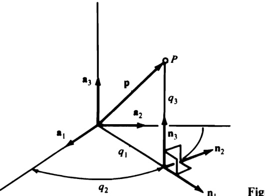
where f_{r} is a function of q_{1},q_{2},q_{3} , and \bar{\mathbf{u}}_{r} is a unit vector. If \mathbf{u}_{1},\,\mathbf{n}_{2} , and \triangledown_{3} are mutually perpendicular, then q_{1},\,q_{2} , and \boldsymbol{q}_{3} are called orthogonal curvilinear coordinates. For instance, suppose that q_{1},\,q_{2} , and \boldsymbol{q}_{3} measure two distances and an angle as indicated in Fig. 2.15.1. Then

{\bf p}=q_{1}\cos q_{2}{\bf a}_{1}+q_{1}\sin q_{2}{\bf a}_{2}+q_{3}{\bf a}_{3}

so that

\begin{array}{r l}&{\displaystyle\frac{\partial{\bf p}}{\partial q_{1}}=\cos q_{2}{\bf a}_{1}+\sin q_{2}{\bf a}_{2}}\\ &{\displaystyle\frac{\partial{\bf p}}{\partial q_{2}}=-q_{1}\sin q_{2}{\bf a}_{1}+q_{1}\cos q_{2}{\bf a}_{2}}\\ &{\displaystyle\frac{\partial{\bf p}}{\partial q_{3}}={\bf a}_{3}}\end{array}

and the functions f_{r} and unit vectors n, (r=1,2,3) appearing in Eqs. (24) can be identified as

\begin{array}{r l}{f_{1}\,=\,1\quad}&{{}\,\mathfrak{n}_{1}\,=\,\cos\,q_{2}\,\mathfrak{a}_{1}\,+\,\sin\,q_{2}\,\mathfrak{a}_{2}\,}\\ {\,\overset{(26)}{\,=\,}}&{{}\quad\mathfrak{n}_{2}\,=\,-\,\sin\,q_{2}\,\mathfrak{a}_{1}\,+\,\cos\,q_{2}\,\mathfrak{a}_{2}\,}\\ {\,\overset{(27)}{\,=\,}}&{{}\quad\mathfrak{n}_{3}\,=\,\mathfrak{a}_{3}\,}\\ {\,\overset{(28)}{\,=\,}}&{{}\quad\mathfrak{n}_{3}\,=\,\mathfrak{a}_{3}}\end{array}

Moreover, it follows from Eqs. (29)-(31) that

\mathbf{n}_{1}\cdot\mathbf{n}_{2}=\mathbf{n}_{2}\cdot\mathbf{n}_{3}=\mathbf{n}_{3}\cdot\mathbf{n}_{1}=0

which means that \mathbb{n}_{1},\,\mathbb{n}_{2} , and \mathfrak{n}_{3} are mutually perpendicular, as indicated in Fig. 2.15.1. Consequently, q_{1},\ q_{2} , and \pmb q_{3} are orthogonal curvilinear coordinates of \pmb{P} in \pmb{A}

When q_{r} (r=1,2,3) are orthogonal curvilinear coordinates of \pmb{P} in \pmb{A} the acceleration a of \pmb{P} in \pmb{A} can be expressed as

{\mathbf a}=a_{1}{\ \mathbf n}_{1}+a_{2}{\ \mathbf n}_{2}+a_{3}{\ \mathbf n}_{3}

where \mathbb{n}_{\ast} (r=1,2,3) ) are the unit vectors appearing in Eqs. (24). To find an expression for a, (r=1,2,3) in terms of f_{1},f_{2},f_{3} and \boldsymbol{q}_{1},\boldsymbol{q}_{2},\boldsymbol{q}_{3} , one can employ Eqs. (2) after noting that the velocity \mathbf{v} of \pmb{P} in \pmb{A} is given by

{\bf v}\!\!\!\!\!\!\!\!\!\!\!\!\!\!\!\!=\!\!\!\!\!\!\!\!\!\!\!\frac{d{\bf p}}{d t}\!\!\!\!\!\!\!\!\!\!\!\!\!\!\!\!\!\!\!\!=\!\!\!\!\!\!\!\!\!\!\!\!\frac{3}{(1.9.1)}\,\!\!\!\!\!\!\!\!\!\!\!\!\!\!=\!\!\!\!\!\!\!\!\!\!\frac{3}{2}\,\!\!\!\!\!\!\!\!\!\!\frac{\partial{\bf p}}{\partial q_{r}}\,\!\!\!\!\!\!\!\!\!\!\!\!\dot{q}_{r}\!\!\!\!\!\!\!\!\!\!\!\!\!\!=\!\!\!\!\!\!\!\!\!\!\sum_{(2.6.1)}^{}f_{r}\dot{q}_{r}{\bf n}_{r}

so that, if \pmb{u}_{\pmb{r}} is defined as in Eqs. (1), then

\mathbf{v}\ =\sum_{\left(34\right)}^{3}\int_{r}u_{r}\mathbf{n}_{r}

which means that

\begin{array}{r}{\pmb{\mathrm{v}}_{r}\quad=\quad f_{r}\,\pmb{\mathrm{n}}_{r}\qquad(r=1,2,3)}\end{array}

and

\mathbf{v}_{1}\cdot\mathbf{a}=f_{1}\mathbf{n}_{1}\cdot(a_{1}\mathbf{n}_{1}+a_{2}\mathbf{n}_{2}+a_{3}\mathbf{n}_{3})=a_{1}f_{1}

But

\pmb{\mathrm{v}}_{1}\cdot\pmb{\mathrm{a}}=\frac{1}{2}\left(\frac{d}{d t}\;\frac{\partial\pmb{\mathrm{v}}^{2}}{\partial\dot{q}_{1}}-\frac{\partial\pmb{\mathrm{v}}^{2}}{\partial q_{1}}\right)

and

v^{2}\ =\ \sum_{(34)\ r\,=\,1}^{3}\ (f_{r}\dot{q}_{r})^{2}

so that

\frac{\partial\mathbf{v}^{2}}{\partial\dot{q}_{1}}\,=\,2\,{f_{1}}^{2}\dot{q}_{1}\qquad\frac{\partial\mathbf{v}^{2}}{\partial q_{1}}\,=\,2\,\sum_{s\,=\,1}^{3}\,f_{s}\frac{\partial f_{s}}{\partial q_{1}}\,\dot{q}_{s}^{\,2}

and

\boldsymbol{\mathbf{v}}_{1}\cdot\boldsymbol{\mathbf{a}}\underset{(38,40)}{=}\frac{d}{d t}(f_{1}^{\ 2}\dot{q}_{1})-\sum_{s=1}^{3}f_{s}\frac{\partial f_{s}}{\partial q_{1}}\dot{q}_{s}^{\ 2}

Substituting from Eq. (41) into Eq. (37) and solving for \pmb{a}_{1} , one thus finds that \pmb{a}_{1} is given by

a_{1}=\frac{1}{f_{1}}\left[\frac{d}{d t}({f_{1}}^{2}\dot{q}_{1})-\sum_{s=1}^{3}f_{s}\frac{\partial f_{s}}{\partial q_{1}}\,\dot{q}_{s}^{~2}\right]

and, after using similar processes in connection with {\mathfrak{a}}_{2} and {\pmb a}_{\pmb3} , one can conclude that

a_{r}={\frac{1}{f_{r}}}\left[{\frac{d}{d t}}\left({f_{r}}^{2}{\dot{q}}_{r}\right)-\sum_{s=1}^{3}\;f_{s}{\frac{\partial f_{s}}{\partial q_{r}}}{\dot{q}_{s}}^{2}\right]\ \ \ \ \ (r=1,2,3)

To illustrate the use of this quite general formula, we return to the orthogonal curvilinear coordinates q_{1},\,q_{2},\,q_{3} introduced in Eq. (25). Expressions for f_{r}\,(r=1,2,3) available in Eqs. (29)-(31) permit us to write

\frac{d}{d t}\bigl(\,f_{1}^{\ 2}\dot{q}_{1}\bigr)\ =\ \ddot{q}_{1}\qquad\frac{\partial f_{1}}{\partial q_{1}}\ =\ 0\qquad\frac{\partial f_{2}}{\partial q_{1}}\ =\ 1\qquad\frac{\partial f_{3}}{\partial q_{1}}\ =\ 0

and, therefore,

a_{1}\mathop{=}_{(43,44)}\ddot{q}_{1}-q_{1}\dot{q}_{2}{}^{2}

Similarly,

\frac{d}{d t}({f_{2}}^{2}\dot{q}_{2})\mathop{=}_{(30)}\frac{d}{d t}({q_{1}}^{2}\dot{q}_{2})\qquad\frac{\partial f_{s}}{\partial q_{2}}_{(29-31)}=\quad0\qquad(s=1,2,3)

so that

a_{2}\mathop{=}_{(43,46)}\frac{1}{q_{1}}\frac{d}{d t}\left({q_{1}}^{2}\dot{q}_{2}\right)

and

\frac{d}{d t}(f_{3}{}^{2}{\dot{q}}_{3})\,=\,\ddot{q}_{3}\qquad\frac{\partial f_{s}}{\partial q_{3}}\mathop{=}_{(29-31)}0\qquad(s\,=\,1,2,3)

which means that

a_{3}\mathop{=}_{(43,48)}\ddot{q}_{3}

Thus, we now can express the acceleration of \pmb{P} in \pmb{A} as

\mathbf{a}\;=\;(\ddot{q}_{1}\,-\,q_{1}\dot{q}_{2}{}^{2})\mathbf{n}_{1}+\frac{1}{q_{1}}\frac{d}{d t}\,({q_{1}}^{2}\dot{q}_{2})\mathbf{n}_{2}\,+\,\ddot{q}_{3}\,\mathbf{n}_{3}

MASS DISTRIBUTION

The motion that results when forces act on a material system depends not only on the forces, but also on the constitution of the system. In particular, the manner in which mass is distributed throughout a system generally affects the behavior of the system. For example, suppose that a rod is supported at one end by a fixed horizontal pin and that a relatively heavy particle is attached at a point of the rod, so that together the rod and the particle form a pendulum. The frequency of the oscillations that ensue when the pendulum is released from rest after having been displaced from the vertical depends on the location of the particle along the rod, that is, on the manner in which mass is distributed throughout the pendulum.

For the purpose of certain analyses, it is unnecessary to know in detail how mass is distributed throughout each of the bodies forming a system; all one needs to know for each body is the location of the mass center, as well as the values of six quantities called inertia scalars. The subject of mass center location is considered in Secs. 3.1 and 3.2. Products of inertia and moments of inertia, which are inertia scalars, are defined in Sec. 3.3 in terms of quantities called inertia vectors. Sections 3.4-3.7 deal with the evaluation of inertia scalars, in which connection inertia matrices and inertia dyadics are discussed. A special kind of moment of inertia, called a principal moment of inertia, is introduced in Sec. 3.8. The chapter concludes with an examination of the relationship between principal moments of inertia, on the one hand, and maximum and minimum moments of inertia, on the Other hand.

3.1 MASS CENTER

\boldsymbol{s} is a set of partiles P_{1},...,P_{v} of masses m_{1},\ldots,m_{\nu} respetivly,there exists a unique point s^{*} such that

\sum_{i=1}^{\nu}\,m_{i}\mathbf{r}_{i}=0

where \mathbf{r}_{i} is the position vector from s^{*} to P_{i}\;(i=1,\ldots,\nu).\;S^{*}, , called the mass center of S, can be located as follows. Let ^o be any point whatsoever, and let \pmb{{\mathsf{p}}_{i}} be the position vector from ^o to P_{i}\;(i=1,\ldots,\nu) Then \mathfrak{p}^{\ast} , the position vector from ^o to s^{*} , is given by

\mathbf{p}^{*}={\frac{\displaystyle\sum_{i=1}^{\nu}m_{i}\mathbf{p}_{i}}{\displaystyle\sum_{i=1}^{\nu}m_{i}}}

Derivation _ With \mathbf{p_{i}} as defined, introduce a point \tilde{s}, let \tilde{\pmb{\uprho}} be the position vector from o to \tilde{s}, and let \tilde{\mathbf{r}}_{i} be the position vector from \tilde{s} to P_{i}\left(i=1,\ldots,\nu\right) .Then

\tilde{\mathbf{r}}_{i}=\mathbf{p}_{i}-\tilde{\mathbf{p}}\qquad(i=1,\ldots,\nu)

and

\begin{array}{c}{{\displaystyle\sum_{i=1}^{v}m_{i}\tilde{\mathbf{r}}_{i}=\sum_{\scriptscriptstyle(3)\atop i=1}^{v}m_{i}\mathbf{p}_{i}-\sum_{\scriptscriptstyle i=1}^{v}m_{i}\tilde{\mathbf{p}}}}\\ {{\displaystyle=\sum_{i=1}^{v}m_{i}\mathbf{p}_{i}-\left(\sum_{\scriptscriptstyle i=1}^{v}m_{i}\right)\tilde{\mathbf{p}}}}\end{array}

Set the right-hand member of this equation equal to zero, solve the resulting equation for {\widetilde{\mathfrak{p}}}, and call the value of \tilde{\pmb{\uprho}} thus obtained \mathbb{P}^{*} . This produces Eq. (2). Next, replace \tilde{\pmb{\uprho}} with \boldsymbol{\mathbf{p}}^{*} in Eq. (3) and let \pmb{\mathrm{r}}_{i} denote the resulting value of {\widetilde{\mathbf{r}}}_{i} . Then \tilde{\mathbf{r}}_{i} may be replaced with \mathbf{r}_{i} in Eq. (4) whenever \tilde{\pmb{\uprho}} is replaced with \mathsf{\pmb{p}}^{\ast} , and under these circumstances Eq. (4) reduces to Eq. (1).

Example A process called “static balancing" consists of adding matter to, or removing matter from, an object (e.g., an automobile wheel) in such a way as to minimize the distance from the mass center of the new object thus created to a specified line (e.g., the axle of the wheel). Consider, for instance, a set of three particles P_{1},P_{2},P_{3} situated at corners of a cube as shown in Fig. 3.1.1 and having masses m, 2m, 3m, respectively. The mass center of this set of particles does not lie on line \pmb{A B} , but, by replacing \boldsymbol{P_{3}} with a particle Q of mass \mu and choosing \mu suitably, one can minimize the distance from line \pmb{A B} to the mass center s^{*} of the set s of particles P_{1},P_{2} , and \pmb{Q}_{\mathrm{{*}}} To determine \pmb{\mu}_{:} introduce \mathsf{\pmb{p}}^{\ast} as the position vector from \pmb{A} to the mass center s^{*} of S, let n be a unit vector directed as shown in Fig. 3.1.1, and note that D^{2} , the square of the distance \pmb{D} from s^{*} to line A B , is given by

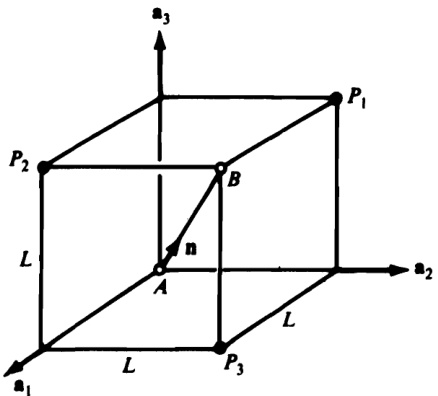
Figure 3.1.1

D^{2}=({\bf p}^{*}\times{\bf\delta n})^{2}

Now, if {\bf a}_{1},{\bf a}_{2},{\bf a}_{3} are unit vectors directed as in Fig. 3.1.1, then

\mathbf{p^{*}}={\frac{m(\mathbf{a}_{2}+\mathbf{a}_{3})+2m(\mathbf{a}_{3}+\mathbf{a}_{1})+\mu(\mathbf{a}_{1}+\mathbf{a}_{2})}{3m+\mu}}L

while

\mathfrak{n}=\frac{\mathfrak{a}_{1}+\mathfrak{a}_{2}+\mathfrak{a}_{3}}{\sqrt{3}}

Consequently,

D^{2}\underset{(5-7)}{=}\frac{2L^{2}(\mu^{2}-3\mu m+3m^{2})}{3(3m+\mu)^{2}}

and, since a value of \pmb{\mu} that minimizes \pmb{D} must satisfy the requirement

\frac{d D^{2}}{d\mu}=0

it may be verified that \mu=5m/3 . In accordance with Eq. (8), the associated (minimum) distance from line \pmb{A}\pmb{B} to s^{*} is equal to L/\sqrt{42}

3.2 CURVES, SURFACES, AND SOLIDS

When a body \pmb{B} is modeled as matter distributed along a curve, over a surface, or throughout a solid, there exists a unique point B^{*} such that

\int_{{\cal F}}\rho{\bf r}\,d\tau=0

where \pmb{\rho} is the mass density (ie., the mass per unit of length, area, or volume) f \pmb{{\cal B}} at a generic point \pmb{P} B,\,\mathfrak{r} is the position vector from \pmb{{\cal B}}^{\ast} P,d\tau is the length, area, or volume of a differential element of the figure \pmb{F} (curve, surface, or solid) occupied by \pmb{B}. and the integration is extended throughout \pmb{F},\pmb{B}^{\ast} , called the mass center of \pmb{B} . can be located as follows. Let ^o be any point whatsoever, and let p be the position vector from o to P Then \mathbf{p}^{*} , the position vector from o to B^{*} ， is given by

\mathbf{p}^{*}={\frac{\displaystyle\int_{F}\rho\mathbf{p}\,d\tau}{\displaystyle\int_{F}\rho\,d\tau}}

The lines of reasoning leading to Eqs. (1) and (2) are analogous to those followed in connection with Eqs.(3.1.1) and (3.1.2).

When \rho varies from point to point of \boldsymbol{B} , the integrals appearing in Eq. (2) generally must be worked out by the analyst who wishes to iocate B^{*} ;but when B isa uniformbody,thatis,when \rho isindependentof thepositionof P in \boldsymbol{B} ,then the desired informationfrequently isreadily available,for B^{*} then coincides with the centroidof thefigure \boldsymbol{F} occupiedby \boldsymbol{B} ；the centroids of many figures have been found(byintegration),and the results have been recorded,as inAppendix I. Thisinformationmakes itpossible tolocate,without performing anyintegrations, the mass center of any body \boldsymbol{B} thatcanberegarded ascomposedsolelyof uniform bodies B_{1},\ldots,B_{\nu} whose masses and mass center locations are known.Under these circumstances, the mass center of B coincides with the mass center of a (fictitious) set of particles (see Sec. 3.1) whose masses are those of B_{1},\dots,B_{\nu} ， and which are situated at the mass centers of B_{1},\dots,B_{\nu} ,respectively.

Example Figure3.2.1 shows a body B consisting ofa wire, E F G attachedto apiece of sheetmetal, E G H (Thelines X_{1},X_{2},X_{3} are mutually perpendicular.) The mass of the sheet metal is 10 times that of the wire.

To locate the mass center B^{*} of B ,welet B_{1} and B_{2} be bodies formed by matterdistributeduniformly alongthestraightline E F and the circular curve F G ,respectively, and model B_{3} ,thesheetmetalportionof B ,asmatter distributeduniformlyovertheplanetrianguiarsurface E G H. The mass centers of B_{1},B_{2} and B_{3} ,found byreferencetoAppendix I,arethepoints B_{1},\,^{*},B_{2},\,^{*} and {B_{3}}^{*} inFig.3.2.2,and themasses m_{1},m_{2} ,and m_{3} Oof B_{1},B_{2} and B_{3} aretakentobe

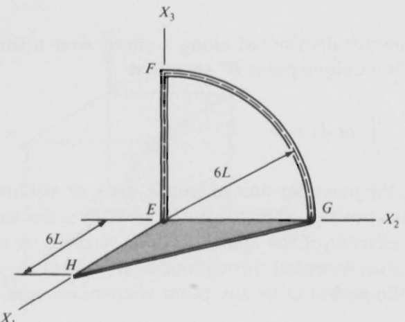
Figure 3.2.1

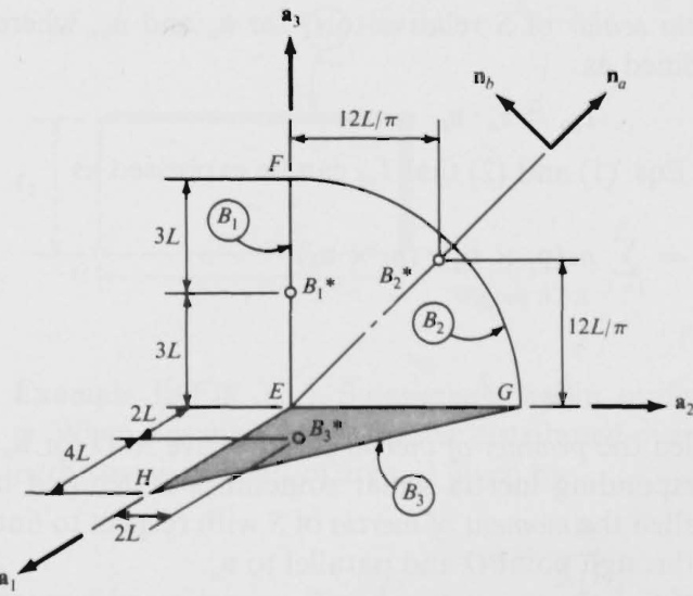
Figure 3.2.2

m_{1}=m\qquad m_{2}={\binom{\pi}{2}}m\qquad m_{3}=10{\bigg(}1+{\frac{\pi}{2}}{\bigg)}m

where m is arbitrary.In accordance with Eq.(3.1.2),the position vector \mathbf{p}^{*} from point E to the mass center of three particles situated at B_{1}^{\mathrm{~*~}},B_{2}^{\mathrm{~\*~}} and {B_{3}}^{*} and having masses m_{1},m_{2} ,and m_{3} ,respectively,isgivenby

\begin{array}{r l}&{\mathbf{p}^{*}=\frac{m_{1}(3L\mathbf{a}_{3})\,+\,m_{2}[(12L/\pi)\mathbf{a}_{2}\,+\,(12L/\pi)\mathbf{a}_{3}]\,+\,m_{3}(2L\mathbf{a}_{1}\,+\,2L\mathbf{a}_{2})}{m_{1}\,+\,m_{2}\,+\,m_{3}}}\\ &{\quad=\underline{{L}}\,\frac{20(1\,+\,\pi/2)\mathbf{a}_{1}\,+\,[6\,+\,20(1\,+\,\pi/2)]\mathbf{a}_{2}\,+\,9\mathbf{a}_{3}}{11(1\,+\,\pi/2)}}\\ &{\quad=(1.82\mathbf{a}_{1}+2.03\mathbf{a}_{2}\,+\,0.318\mathbf{a}_{3})L}\end{array}

The vector \mathbf{p}^{*} is theposition vector from E to B^{*} the mass center of B_{e} and Eq.(4) shows that B^{*} lies neither on the wire nor on the sheet metal portion of \boldsymbol{B}

3.3INERTIA VECTOR,INERTIA SCALARS

{\cal{S}} is a set of partiles P_{1},\dots,P_{\nu} of masses m_{1},\ldots,m_{\nu} respectively, \mathbf{p}_{i} isthe position vector from a point o to P_{i}\,(i=1,\dots,\nu) and {\bf n}_{a} is a unit vector, then a vector {\bf I}_{a} calledtheinertiavectorof s relativeto {\upsilon} for {\mathfrak{n}}_{a} , is defined as

\mathbf{I}_{a}\triangleq\sum_{i=1}^{\nu}m_{i}\mathbf{p}_{i}\times(\mathbf{n}_{a}\times\mathbf{p}_{i})

A scalar {\cal I}_{a b} , called the inertia scalar of \boldsymbol{s} relative to ^o for \pmb{\mathrm{\scriptscriptstyleR}}_{\pmb{a}} and \pmb{\mathrm{\scriptscriptstylem}}_{b} , where \mathbb{n}_{b} like \mathbb{n}_{\pmb{\alpha}} , is a unit vector, is defined as

I_{a b}\triangleq\mathbf{I}_{a}\!\cdot\mathbf{n}_{b}

It follows immediately from Eqs. (1) and (2) that \boldsymbol{I}_{a b} can be expressed as

I_{a b}=\sum_{i=1}^{\nu}m_{i}({\bf p}_{i}\,\times\,{\bf n}_{a})\cdot({\bf p}_{i}\,\times\,{\bf n}_{b})

and this shows that

I_{a b}=I_{b a}

When \mathbb{n}_{b}\neq\mathbb{n}_{a} ， {\cal I}_{o b} is called the product of inertia of S relative to ^o for \mathbb{n}_{\pmb{a}} and \pmb{\mathrm{u}}_{\pmb{b}} . When \mathbb{n}_{b}=\mathbb{n}_{a} , the corresponding inertia scalar sometimes is denoted by \pmb{I_{a}} (rather than by I_{a a}) , and is called the moment of inertia of S with respect to line L_{a} where L_{a} is the line passing through point ^o and parallel to \mathbb{n}_{a}

The moment of inertia of \boldsymbol{s} with respect to a line L_{a} can always be expressed both as

I_{a}=\sum_{i\,=\,1}^{\nu}m_{i}{l_{i}}^{2}

where l_{i} is the distance from \pmb{P_{i}} to line L_{\pmb{\mathscr{a}}} , and as

I_{a}=m k_{a}^{~2}

where m is the total mass of \pmb{S}_{\pmb{\imath}} and k_{a} is a real, non-negative quantity called the radius of gyration of \pmb{s} with respect to line L_{a} . Equation (5) follows from the fact that

I_{a}=\sum_{\scriptstyle(3)\ i=1}^{\nu}m_{i}({\bf p}_{i}\,\times\,{\bf n}_{a})^{2}

and that \mathbf{p}_{i}\times\bar{\mathbf{u}}_{a} has the magnitude l_{i} , the vector \pmb{\mathrm{p}_{i}} being the position vector from a point on L_{a} to \boldsymbol{P_{i}}

Inertia vectors, products of inertia, moments of inertia, and radi of gyration of a body \pmb{B} modeled as matter distributed along a curve, over a surface, or throughout a solid are defined analogously. Specifically, if \pmb{\rho} is the mass density (i.e., the mass per unit of length, area, or volume) of \pmb{B} at a generic point \pmb{P} \pmb{B} , p is the position vector from a point ^o to P,d\tau is the length, area, or volume of a differential element of the figure {\pmb F} (curve, surface, or solid) occupied by \pmb{B}, and \pmb{\mathrm{n}}_{\pmb{a}} and \bigtriangledown_{b} are unit vectors, then Eqs. (1), (2), and (5) give way, respectively, to

\begin{array}{c}{\displaystyle\mathbf{I}_{a}\triangleq\int_{F}\boldsymbol{\rho}\mathbf{p}\,\times\,(\mathbf{n}_{a}\times\,\mathbf{p})\,d\tau}\\ {\displaystyle I_{a b}\triangleq\,\mathbf{I}_{a}\cdot\mathbf{n}_{b}=\int_{F}\boldsymbol{\rho}(\mathbf{p}\,\times\,\mathbf{n}_{a})\cdot(\mathbf{p}\,\times\,\mathbf{n}_{b})\,d\tau}\\ {\displaystyle I_{a}=\int_{F}\boldsymbol{\rho}l^{2}\,d\tau}\end{array}

where l is the distance from \pmb{P} to line L_{a} ; and Eq. (6) applies to \pmb{B} as well as to \pmb{S},

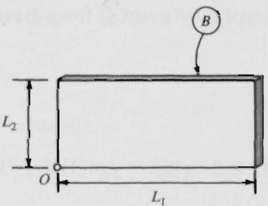
Figure 3.3.1

Example In Fig.3.3.1, B designates a thin,uniform,rectangular plate of mass m. When B ismodeled asmatter distributed over a rectangular surface R then \rho the massper unit of area,is given by

\rho=\frac{m}{L_{1}L_{2}}

while \mathbf{p} thepositionvectorfrompoint o to a genericpoint P of B canbeexpressed as

\mathbf{p}=x_{1}\mathbf{n}_{1}+x_{2}\mathbf{n}_{2}

where x_{1} and x_{2} are distances,and {\bf{u}}_{1} and \mathbf{n}_{2} are unit vectors, as shown in Fig.3.3.2. The inertia vector of \boldsymbol{B} with respect to o for {\mathfrak{w}}_{1} is thus

\begin{array}{l c l}{{{\bf{I}}_{1}^{0}}}&{{=}}&{{\displaystyle\int_{R}\rho\ {\bf{x}}\ ({\bf{n}}_{1}\times{\bf{p}})\,d\tau}}\\ {{\mathrm{{\bf{\sigma}}}_{(1),1}^{=}}}&{{=}}&{{\displaystyle\int_{0}^{L_{2}}\int_{0}^{L_{1}}\frac{m}{L_{1}L_{2}}(x_{1}{\bf{n}}_{1}+x_{2}{\bf{n}}_{2})\times\ \left[{\bf{n}}_{1}\times(x_{1}{\bf{n}}_{1}+x_{2}{\bf{n}}_{2})\right]d x_{1}\ d x_{2}}}\\ {{\mathrm{{\bf{\sigma}}}_{(1),1}^{=}}}&{{=}}&{{\displaystyle\frac{m}{L_{1}L_{2}}\int_{0}^{L_{2}}\int_{0}^{L_{1}}\left(x_{2}^{2}{\bf{n}}_{1}-x_{1}x_{2}{\bf{n}}_{2}\right)d x_{1}\ d x_{2}}}\\ {{\mathrm{{\bf{\sigma}}}=}}&{{\displaystyle\frac{m}{L_{1}L_{2}}\left({\bf{n}}_{1}\int_{0}^{L_{2}}\int_{0}^{L_{1}}x_{2}^{2}\,d x_{1}\,d x_{2}-{\bf{n}}_{2}\int_{0}^{L_{2}}\int_{0}^{L_{1}}x_{1}x_{2}\,d x_{1}\,d x_{2}\right)}}\\ {{\mathrm{{\bf{\sigma}}}=}}&{{\displaystyle\frac{m}{L_{1}L_{2}}\left({\bf{n}}_{1}\frac{L_{1}L_{2}{}^{3}}{3}-{\bf n}_{2}\frac{L_{1}^{1}L_{2}{}^{2}}{4}\right)=m L_{2}\left(\frac{L_{2}}{3}{\bf n}_{1}-\frac{L_{1}}{4}{\bf n}_{2}\right)}}\end{array}

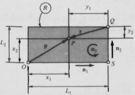
Figure 3.3.2

Similarly, \dot{\mathbf{I}}_{3}{^{Q}!} , the inertia vector of \pmb{B} with respect to point \pmb{Q} for \mathbb{n}_{3} , can be written (see Fig. 3.3.2 for r)

\begin{array}{l}{\displaystyle\mathbf{I}_{3}^{\,Q}=\int_{R}\rho\mathbf{r}\,\times\,(\mathbf{n}_{3}\,\times\,\mathbf{r})\,d\tau}\\ {\displaystyle}\\ {\,=\,\int_{0}^{L_{2}}\int_{0}^{L_{1}}\!\frac{m}{L_{1}L_{2}}(-y_{1}\mathbf{n}_{1}-y_{2}\mathbf{n}_{2})\,\times\big[\mathbf{n}_{3}\times\,(-y_{1}\mathbf{n}_{1}-y_{2}\mathbf{n}_{2})\big]\,d y_{1}\,d y_{2}}\\ {\,=\displaystyle\frac{m}{L_{1}L_{2}}\int_{0}^{L_{2}}\!\int_{0}^{L_{1}}(y_{1}^{\,2}+y_{2}^{\,2})\,d y_{1}\,d y_{2}\,\mathbf{n}_{3}=\frac{m}{3}(L_{1}^{\,2}+L_{2}^{\,2})\mathbf{n}_{3}\quad\qquad(1\to\infty)}\end{array}

With the aid of these results, the inertia scalars I_{1j}^{\mathrm{~\,~}o} and I_{3j}{}^{Q}\,(j=1,2,3) can be formed as

\begin{array}{l l l l l}{{\displaystyle I_{11}{}^{o}={\bf I_{1}}^{o}\cdot{\bf n}_{1}={\frac{m L_{2}{}^{2}}{3}}\quad}}&{{\displaystyle I_{12}{}^{o}{}={}}}&{{\!-{\frac{m L_{1}L_{2}}{4}}}}&{{\displaystyle I_{13}{}^{o}{}={}~0~~~}}&{{\displaystyle(1)}}\\ {{\displaystyle(2)\quad~~~~~~~~~(13)\quad~~}}&{{\displaystyle(2,13)\quad~~}}&{{}}&{{}}\\ {{\displaystyle I_{31}{}^{o}={\bf I_{3}}^{o}\cdot{\bf n}_{1}={}~0\quad}}&{{\displaystyle I_{32}{}^{o}{}={}~0}}&{{\displaystyle I_{33}{}^{o}{}={}~{\frac{m}{(2,14)}}(L_{1}{}^{2}+L_{2}{}^{2})}}\end{array}

Two of these inertia scalars are moments of inertia, namely, {I_{1}}_{1}^{o} and \mathbf{\nabla}I_{33}^{\mathrm{~\,~}0} The first is the moment of inertia of \pmb{B} about line \pmb{o s} ; the second is the moment of inertia of \pmb{B} about the line passing through \pmb{Q} and parallel to \pmb{\mathrm{u}}_{\pmb{3}} ：

3.4 MUTUALLY PERPENDICULAR UNIT VECTORS

Knowledge of the inertia vectors \mathbf{I}_{1},\mathbf{I}_{2},\mathbf{I}_{3} of a body \pmb{B} relative to a point ^o (see Sec. 3.3)for three mutually perpendicular unit vectors \bar{\mathbf{n}}_{1},\bar{\mathbf{n}}_{2},\bar{\mathbf{n}}_{3} enables one to find {\bf I}_{a} , the inertia vector of \pmb{B} relative to o for any unit vector \mathbb{n}_{a} , for

{\bf I}_{a}=\sum_{j=1}^{3}a_{j}{\bf I}_{j}

where a_{1},a_{2},a_{3} are defined as

a_{j}\triangleq\mathfrak{n}_{a}\cdot\mathfrak{n}_{j}\qquad(j=1,2,3)

Similarly, \boldsymbol{I}_{a b} , the inertia scalar of \pmb{B} relative to ^o for \mathbb{n}_{\pmb{a}} and \mathbb{n}_{b} (see Sec. 3.3), can be found easily when the inertia scalars I_{j k}\left(j,k=1,2,3\right) are known, for

I_{a b}=\sum_{j=1}^{3}\sum_{k=1}^{3}a_{j}I_{j k}b_{k}

where

b_{k}\triangleq\mathfrak{n}_{b}\cdot\mathfrak{n}_{k}\qquad(k=1,2,3)

Derivations It follows from Eq. (2) that (see Sec. 1.3)

{\displaystyle{\bf n}_{a}=\sum_{j\,=\,1}^{3}a_{j}{\bf n}_{j}}

Consequently,

\begin{array}{r l}{\displaystyle\mathrm{I}_{a_{\phantom{(}3.3.1)}\,i=1}\quad}&{\displaystyle\sum_{i=1}^{\nu}\,m_{i}\{\boldsymbol{\mathsf{p}}_{i}\times\left(\sum_{j=1}^{3}a_{j}\boldsymbol{\mathsf{n}}_{j}\times\boldsymbol{\mathsf{p}}_{i}\right)}\\ {\displaystyle}&{=\quad\displaystyle\sum_{j=1}^{3}a_{j}\,\sum_{i=1}^{\nu}m_{i}\boldsymbol{\mathsf{p}}_{i}\times(\boldsymbol{\mathsf{n}}_{j}\times\boldsymbol{\mathsf{p}}_{i})}\\ {\displaystyle}&{=\quad\displaystyle\sum_{j=1}^{3}a_{j}\boldsymbol{\mathsf{I}}_{j}}\end{array}

which establishes the validity of Eq. (1). As for Eq. (3), note that Eq. (4) implies that (see Sec. 1.3)

{\mathbf{n}}_{b}=\sum_{k\,=\,1}^{3}b_{k}\,{\mathbf{n}}_{k}

Hence,

\begin{array}{r l}{{\displaystyle I_{a b}\quad=\quad\left(\sum_{j=1}^{3}a_{j}\mathbb{I}_{j}\right)\cdot\sum_{k=1}^{3}b_{k}\mathbb{n}_{k}}}&{{}}\\ {{\displaystyle=\quad\sum_{j=1}^{3}\sum_{k=1}^{3}a_{j}\mathbb{I}_{j}{\cdot\cdot\mathbb{n}_{k}}b_{k}=\sum_{j=1}^{3}\sum_{k=1}^{3}a_{j}I_{j k}b_{k}}}&{{}}\end{array}

Example Table 3.4.1 shows the inertia scalars I_{j k} of \pmb{{\cal B}} relative to _o for {\bf\Delta}\equiv_{j} and {\mathfrak{n}}_{k}\,(j,k=1,2,3) ,where \pmb{B} is the rectangular plate considered in the example in Sec. 3.3. To find the moment of inertia of \pmb{B} withrespecttoline o Q in Fig. 3.3.2, let \mathbb{n}_{\pmb{a}} be a unit vector parallel to this line, so that

\mathtt{n}_{a}=\frac{L_{1}\mathfrak{n}_{1}+L_{2}\mathfrak{n}_{2}}{({L_{1}}^{2}+{L_{2}}^{2})^{1/2}}

Table 3.4.1

<html>

1k	1	2	3
1	mL22/3	-mL,L2/4	0
2	-mL,L2/4	mL,2/3	0
3	0	0	m(L,² + L2²)/3

</html>

which means that, in accordance with Eq. (2)

a_{1}=\frac{L_{1}}{({L_{1}}^{2}+{L_{2}}^{2})^{1/2}}\qquad a_{2}=\frac{L_{2}}{({L_{1}}^{2}+{L_{2}}^{2})^{1/2}}\qquad a_{3}=0

With b_{k}=a_{k}\,(k=1,2,3) , Eq. (3) then yields [see also Eq. (3.3.4)]

{\begin{array}{r l}&{I_{a}\,=\,{a_{1}}^{2}I_{11}\,+\,{a_{2}}^{2}I_{22}\,+\,{a_{3}}^{2}I_{33}\,+\,2({a_{1}}{a_{2}}I_{12}\,+\,{a_{2}}{a_{3}}I_{23}\,+\,{a_{3}}{a_{1}}I_{31})}\\ &{\quad\,=\,{\cfrac{{L_{1}}^{2}I_{11}\,+\,{L_{2}}^{2}I_{22}\,+\,2L_{1}L_{2}\,I_{12}}{{L_{1}}^{2}\,+\,{L_{2}}^{2}}}}\end{array}}

and use of Table 3.4.1 leads to

I_{a}={\frac{m L_{1}{}^{2}{L_{2}}^{2}/3+m L_{1}{}^{2}{L_{2}}^{2}/3-m L_{1}{}^{2}{L_{2}}^{2}/2}{{L_{1}}^{2}+{L_{2}}^{2}}}={\frac{m(L_{1}L_{2})^{2}}{6({L_{1}}^{2}+{L_{2}}^{2})}}

3.5 INERTIA MATRIX, INERTIA DYADIC

The inertia scalars I_{j k} of a set \pmb{s} of particles relative to a point ^o for unit vectors {\pmb\mathrm{n}}_{j} and {\mathfrak{n}}_{k}\left(j,k=1,\right. 2, 3) can be used to define a square matrix \pmb{I}. called the inertia matrix of \boldsymbol{s} relative to ^o for \tilde{\mathbf{n}}_{1},\tilde{\mathbf{n}}_{2},\tilde{\mathbf{n}}_{3} , as follows:

I\triangleq{\left[\begin{array}{l l l}{I_{11}}&{I_{12}}&{I_{13}}\\ {I_{21}}&{I_{22}}&{I_{23}}\\ {I_{31}}&{I_{32}}&{I_{33}}\end{array}\right]}

Suppose that \mathbf{n}_{1},\,\mathbf{n}_{2},\,\mathbf{n}_{3} are mutually perpendicular and that row matrices \pmb{a} and \pmb{b} are defined as

a\triangleq[a_{1}\quad a_{2}\quad a_{3}]\qquad b\triangleq[b_{1}\quad b_{2}\quad b_{3}]

where a_{1},a_{2},a_{3} and b_{1},b_{2},b_{3} are given by Eqs. (3.4.2) and (3.4.4), respectively. Then it follows immediately from Eq. (3.4.3) and the rules for multiplication of matrices that \pmb{I_{a b}} , the inertia scalar of \pmb{s} relative to ^o for \mathbb{n}_{a} and \mathbb{n}_{b} , is given by

\boldsymbol{I_{a b}}=a\boldsymbol{I}\boldsymbol{b}^{\tau}

where b^{\pmb{r}} is the transpose of \pmb{b} , that is, the column matrix having \pmb{b}_{i} as the element in the ith row (i=1,2,3) 0. Equation (3) is useful when inertia scalars are evaluated by means of machine computations and matrix multiplication routines are readily available.

The set \pmb{s} does not possess a unique inertia matrix relative to ^o , for, if {\mathfrak{n}}_{1}^{\prime} ， \mathbb{n}_{2}^{\prime},\,\mathbb{n}_{3}^{\prime} are mutually perpendicular unit vectors other than \mathbf{n}_{1},\,\mathbf{n}_{2},\,\mathbf{n}_{3} , and \pmb{I^{\prime}} is defined as

I^{\prime}\triangleq{\left[\begin{array}{l l l}{I_{11^{'}}}&{I_{12^{'}}}&{I_{13^{'}}}\\ {I_{21^{'}}}&{I_{22^{'}}}&{I_{23^{'}}}\\ {I_{31^{'}}}&{I_{32^{'}}}&{I_{33^{'}}}\end{array}\right]}

where I_{j k}^{\ \ \prime}\left(j,k=1,2,3\right) are the inertia scalars of S relative to ^o for \mathbf{n}_{j}^{\prime} and {\mathop{\mathbf{n}}}_{k}^{\prime} then r , like \pmb{I} , is an inertia matrix of S relative to o , but \pmb{I} and I^{\prime} are by no means equal to each other. Hence, when working with inertia matrices, one must keep in mind that each such matrix is associated with a specific vector basis. By way of contrast, the use of dyadics enables one to deal with certain topics involving inertia vectors and/or inertia scalars in a basis-independent way. To acquaint the reader with dyadics, we begin by focusing attention on two vectors, u and \mathbf{v}. given by

and

\begin{array}{r}{\mathbf{u}=\mathbf{w}\cdot\mathbf{a}\mathbf{b}+\mathbf{w}\cdot\mathbf{c}\mathbf{d}+\cdots}\\ {\ }\\ {\mathbf{v}=\mathbf{a}\mathbf{b}\cdot\mathbf{w}+\mathbf{c}\mathbf{d}\cdot\mathbf{w}+\cdots}\end{array}

respectively, where a, b, c, d, ..., and \mathbf{w} are any vectors whatsoever. Equations (5) and (6) can be rewritten as

\mathbf{u}=\mathbf{w}\cdot(\mathbf{ab}+\mathbf{cd}+\cdots)

and

\mathbf{v}=(\mathbf{ab}+\mathbf{cd}+\cdots)\cdot\mathbf{w}

if it is understood that the right-hand members of Eqs. (7) and (8) have the same meanings as those of Eqs. (5) and (6), respectively. Furthermore, if the quantity within parentheses in Eqs. (7) and (8) is denoted by Q, that is, if \mathbf{Q} is defined as

\mathbf{Q}\triangleq\mathbf{ab}+\mathbf{cd}+\cdots

then Eqs. (7) and (8) give way to

\mathbf{u}=\mathbf{w}\cdot\mathbf{Q}

and

\mathbf{v}=\mathbf{Q}\cdot\mathbf{w}

respectively; Q is called a dyadic; and Eqs. (5), (9), and (10) constitute a definition of scalar premultiplication of a dyadic with a vector, while Eqs. (6),(9), and (11) define the operation of scalar postmultiplication of a dyadic with a vector. In summary, then, a dyadic is a juxtaposition of vectors as in the right-hand member of Eq. (9), and scalar multiplication (pre- or post-) of a dyadic with a vector produces a vector.

A rather special dyadic U, called the unit dyadic, comes to light in connection with Eq. (1.3.3), which suggests the defnition

\mathbf{U}\triangleq\mathbf{a}_{1}\mathbf{a}_{1}+\mathbf{a}_{2}\mathbf{a}_{2}+\mathbf{a}_{3}\mathbf{a}_{3}

where {\mathfrak{a}}_{1},\,{\mathfrak{a}}_{2},\,{\mathfrak{a}}_{3} are mutually perpendicular unit vectors. In accordance with Eqs. (5), (9), and (10),

\qquad\mathbf{v}\cdot\mathbf{U}\ =\ \mathbf{v}\cdot\mathbf{a}_{1}\mathbf{a}_{1}\,+\,\mathbf{v}\cdot\mathbf{a}_{2}\,\mathbf{a}_{2}\,+\,\mathbf{v}\cdot\mathbf{a}_{3}\,\mathbf{a}_{3}\quad=\quad\mathbf{v}

Moreover, it follows from Eqs. (6), (9), and (11) that

\mathbf{U}\cdot\mathbf{v}\ =\ \mathbf{a}_{1}\mathbf{a}_{1}\cdot\mathbf{v}\ +\ \mathbf{a}_{2}\mathbf{a}_{2}\cdot\mathbf{v}\ +\ \mathbf{a}_{3}\mathbf{a}_{3}\cdot\mathbf{v}\ \underset{(1.3.3)}{=}\mathbf{v}

In other words, \mathbf{U} is a dyadic whose scalar product (pre- or post-) with any vector is equal to the vector itself.

Returning to the subject of inertia vectors and inertia scalars, let us consider the inertiavector {\bf I}_{a} , defined as in Eq. (3.3.1). This can be expressed as

\begin{array}{r l}{\displaystyle\mathbf{I}_{a}\ =\ }&{\displaystyle\sum_{(3.3.1)\ i=1}^{\nu}\,m_{i}(\mathbf{n}_{a}\,{\mathbf{p}_{i}}^{2}\,-\,\mathbf{n}_{a}\cdot\mathbf{p}_{i}\,\mathbf{p}_{i})}\\ {\,=\ }&{\displaystyle\sum_{i=1}^{\nu}m_{i}(\mathbf{n}_{a}\cdot\mathbf{U}{\mathbf{p}_{i}}^{2}\,-\,\mathbf{n}_{a}\cdot\mathbf{p}_{i}\,\mathbf{p}_{i})}\end{array}

Hence, if a dyadic I is defined as

\mathbf{I}\triangleq\sum_{i=1}^{\nu}m_{i}(\mathbf{U}{\mathbf{p}_{i}}^{2}-\mathbf{p}_{i}\mathbf{p}_{i})

then {\mathbf{I}}_{\pmb{a}} can be expressed as

{\mathbf I}_{a}={\bar{\mathbf{n}}}_{a}\cdot{\mathbf I}

The dyadic I is called the inertia dyadic of S relative to ^o Whenabody \pmb{B} is modeled as matter occupying a figure F (a curve, surface, or solid), then Eq. (16) is replaced with

\mathbf{I}\triangleq\int_{F}\rho(\mathbf{U}\mathbf{p}^{2}-\mathbf{p}\mathbf{p})\,d\tau

where \rho,\,\pmb{\mathrm{p}}, and \pmb{d}\tau have the same meanings as in connection with Eq. (3.3.8).

Dot-multiplication of Eq. (17) with a unit vector \mathbb{n}_{b} leads to

{\bf I}_{a}\cdot{\bf n}_{b}=({\bf n}_{a}\cdot{\bf I})\cdot{\bf n}_{b}

In view of Eq. (3.3.2) and the fact that (\tilde{\mathbf{n}}_{a}\cdot\tilde{\mathbf{I}})\cdot\tilde{\mathbf{n}}_{b}=\tilde{\mathbf{n}}_{a}\cdot(\tilde{\mathbf{I}}\cdot\tilde{\mathbf{n}}_{b}), so that the parentheses in Eq. (19) are unnecessary, one thus finds that the inertia scalar {\cal I}_{a b} canbe expressed as

I_{a b}=\tilde{\mathbf{n}}_{a}\!\cdot\!\mathbf{I}\cdot\!\mathbf{n}_{b}

The inertia dyadic I is said to be basis-independent because its definition, Eq. (16), does not involve any basis vectors. However,it can be expressed in various basis-dependent forms. For example, if \mathbf{n}_{1},\ \mathbf{n}_{2},\ \mathbf{n}_{3} are mutually perpendicular unit vectors, {\bf{I}}_{j} is the inertia vector of \pmb{s} relative to ^o for {\mathfrak{n}}_{j}\,(j=1,2,3) , and I_{j k} is the inertia scalar of S relative to O for n; and nz (j, k = i, 2, 3), then I is given both by

\mathbf{I}=\sum_{j=1}^{3}\mathbf{I}_{j}\mathbf{n}_{j}

and by

\mathbf{I}=\sum_{j=1}^{3}\sum_{k\,=\,1}^{3}I_{j k}\mathbf{n}_{j}\mathbf{n}_{k}

Derivation It may be verifed that a relationship analogous to Eq. (1.3.3) applies to anydyadic \mathbf{Q} ; that is,

\mathbf{Q}=\mathbf{n}_{1}\cdot\mathbf{Q}\bar{\mathbf{n}}_{1}+\bar{\mathbf{n}}_{2}\cdot\mathbf{Q}\bar{\mathbf{n}}_{2}+\bar{\mathbf{n}}_{3}\cdot\mathbf{Q}\bar{\mathbf{n}}_{3}

Consequently,

\begin{array}{r l}&{\mathbf{I}\,=\,{\boldsymbol{\mathbf{n}}}_{1}\cdot\mathbf{I}{\boldsymbol{\mathbf{n}}}_{1}\,+\,{\boldsymbol{\mathbf{n}}}_{2}\cdot\mathbf{I}{\boldsymbol{\mathbf{n}}}_{2}\,+\,{\boldsymbol{\mathbf{n}}}_{3}\cdot\mathbf{I}{\boldsymbol{\mathbf{n}}}_{3}}\\ &{\,=\,\mathbf{I}_{1}{\boldsymbol{\mathbf{n}}}_{1}\,+\,\mathbf{I}_{2}\,{\boldsymbol{\mathbf{n}}}_{2}\,+\,\mathbf{I}_{3}\,{\boldsymbol{\mathbf{n}}}_{3}}\\ &{\,(17)}\end{array}

in agreement with Eq. (21). As for Eq. (22), refer to Eq. (1.3.3) to write

\begin{array}{r l}{\mathbf{I}_{j}}&{=\phantom{-}\mathbf{I}_{j}\cdot\mathbf{n}_{1}\mathbf{n}_{1}+\mathbf{I}_{j}\cdot\mathbf{n}_{2}\mathbf{n}_{2}+\mathbf{I}_{j}\cdot\mathbf{n}_{3}\mathbf{n}_{3}}\\ &{\phantom{=}=\phantom{-}I_{j1}\mathbf{n}_{1}+\phantom{-}I_{j2}\mathbf{n}_{2}+\phantom{-}I_{j3}\mathbf{n}_{3}\qquad(j=1,2,3)}\end{array}

and substitute these expressions for \mathbf{I}_{1},\mathbf{I}_{2} , and \mathbf{I}_{3} into Eq. (24) to obtain

{\begin{array}{r l}{\mathbf{I}=(I_{11}\mathbf{n}_{1}+I_{12}\mathbf{n}_{2}+I_{13}\mathbf{n}_{3})\mathbf{n}_{1}}&{}\\ {+\mathbf{\Gamma}(I_{21}\mathbf{n}_{1}+I_{22}\mathbf{n}_{2}+I_{23}\mathbf{n}_{3})\mathbf{n}_{2}}&{}\\ {+\mathbf{\Gamma}(I_{31}\mathbf{n}_{1}+I_{32}\mathbf{n}_{2}+I_{33}\mathbf{n}_{3})\mathbf{n}_{3}}\end{array}}

which is seen to agree with Eq. (22).

Example If S is a set of particles P_{1},\dots,P_{v} of masses \pmb{m}_{1},\dots,\pmb{m}_{\nu} , respectively, moving in a reference frame \pmb{A} with velocities A_{\mathbf{v}}P_{1},\ldots,A_{\mathbf{v}}P_{\nu} (see Sec. 2.6), then a vector \pmb{A}\mathbf{H}^{\pmb{S}/o} , called the angular momentum of \boldsymbol{s} relative to ^o in \pmb{A} , is defined as

{}^{A}\mathbf{H}^{S/O}\triangleq\sum_{i=1}^{\nu}m_{i}\mathbf{p}_{i}\times{}^{A}\mathbf{v}^{P_{i}}

where \pmb{\mathrm{p}_{i}} is the position vector from a point ^o to P_{i}\,(i=1,\ldots,\nu) The point o need not befixed in \pmb{A} ; for example, it can be the mass center s^{*} of S,in which case \pmb{A}\pmb{\mathrm{H}}^{\pmb{S}/\pmb{O}} becomes \pmb{A}\mathbf{H}^{\pmb{S}/\pmb{S}^{\star}} and is called the central angular momentum of S in \pmb{A}

If the particles of \pmb{s} form a rigid body \pmb{B}. then \mathbf{H}_{\mathrm{:}} the central angular momentum of \pmb{B} in \pmb{A} , can be expressed as

\mathbf{H}=\mathbf{I}\cdot\mathbf{\omega}

where I, called the central inertia dyadic of \pmb{B} is the inertia dyadic of \pmb{B} relative to the mass center \pmb{{\cal B}}^{\ast} of \pmb{B}. and \pmb{\infty} is the angular velocity of \pmb{B} in \pmb{A} To verify

that \mathbf{H} can be written as in Eq. (28), let \mathbf{r}_{i} be the position vector from B^{*} to P_{i} and refer to Eqs. (27) and (2.7.1) to write

\begin{array}{l}{\displaystyle\mathbf{H}=\sum_{i=\,1}^{\,v}\,m_{i}\,\mathbf{r}_{i}\,\times\,\left(\mathbf{\nabla}^{A}\mathbf{v}^{B^{\star}}+\mathbf{\Leftrightarrow}\,\mathbf{\times}\,\mathbf{r}_{i}\right)}\\ {\displaystyle\qquad=\left(\sum_{i=\,1}^{\,v}\,m_{i}\,\mathbf{r}_{i}\right)\,\times\,\mathbf{\mathcal{A}}_{\mathbf{v}}^{\,B^{\star}}+\,\sum_{i=\,1}^{\,v}\,m_{i}\,\mathbf{r}_{i}\,\times\,(\mathbf{\omega}\times\,\mathbf{r}_{i})}\end{array}

Then note that

\sum_{i=1}^{\nu}\,m_{i}\mathbf{r}_{i}\,\mathbf{\phi}_{(3,1,1)}^{\phantom{\nu}}\,0

while

\begin{array}{r l r}{\lefteqn{\sum_{i=1}^{\nu}m_{i}\mathbf{r}_{i}\times(\boldsymbol{\omega}\times\mathbf{r}_{i})=\sum_{i=1}^{\nu}m_{i}(\mathbf{r}_{i}^{\,2}\boldsymbol{\omega}-\mathbf{r}_{i}\mathbf{r}_{i}\cdot\boldsymbol{\omega})}}\\ &{}&{=\displaystyle\sum_{i=1}^{\nu}m_{i}(\mathbf{r}_{i}^{\,2}\mathbf{U}-\mathbf{r}_{i}\mathbf{r}_{i})\cdot\boldsymbol{\omega}\,=\,\mathbf{I}\cdot\boldsymbol{\omega}}\end{array}

\omega_{1},\omega_{2},\omega_{3} are defined as

\omega_{i}\triangleq\omega\cdot\mathbf{n}_{i}\qquad(i=1,2,3)

then it follows directly from Eqs. (28), (22), and (32) that

\begin{array}{r}{\mathbf{H}=\displaystyle\sum_{j=1}^{3}\sum_{k=1}^{3}I_{j k}\mathbf{n}_{j}\mathbf{n}_{k}\cdot\sum_{i=1}^{3}\omega_{i}\mathbf{n}_{i}}\\ {=\displaystyle\sum_{i=1}^{3}\sum_{j=1}^{3}\sum_{k=1}^{3}I_{j k}\omega_{i}\mathbf{n}_{j}\mathbf{n}_{k}\cdot\mathbf{n}_{i}}\end{array}

so that, since \mathbf{u}_{k}\cdot\mathbf{n}_{i} vanishes except when i=k in which case it is equal to unity, \mathbf{H} can be written

\mathbf{H}\ =\ \sum_{(33)\ j=1}^{3}\sum_{k=1}^{3}I_{j k}\omega_{k}\mathbf{n}_{j}

This is a useful relationship. It reduces to the convenient form given in Eq. (2.3.5) if \bar{\bf n}_{1},\bar{\bf n}_{2},\bar{\bf n}_{3} are chosen in such a way that I_{12},I_{23} , and \boldsymbol{I}_{31} vanish. The fact that it is always possible to choose \mathbf{n}_{1},\mathbf{n}_{2},\mathbf{n}_{3} in this way is established in Sec. 3.8.

3.6 PARALLEL AXES THEOREMS

The inertia dyadic \mathbf{I}^{s/o} of a set S of \boldsymbol{\upnu} particles P_{1},\dots,P_{v} relative to a point ^o (see Sec. 3.5) is related in a simple way to the central inertia dyadic \mathbf{I}^{\pmb{S}/\pmb{S}^{\star}} of \pmb{s} that is, the inertia dyadic of S relative to the mass center s^{*} of S. Specifically,

\mathbf{I}^{s/\sigma}=\mathbf{I}^{s/S^{\bullet}}+\mathbf{I}^{s^{\bullet}/\sigma}

where \mathbf{I}^{s\bullet_{/\bullet}} denotes the inertia dyadic relative to ^o of a (fictitious) particle situated at s^{\star} and having a mass equal to the total mass of S. Similarly, if \pmb{I}^{\pmb{S}/\pmb{O}} and I^{\pmb{s}/\pmb{s}^{\star}}

are inertia matrices of S relative to ^o and s^{*} , respectively, for unit vectors \mathbf{n}_{1},\mathbf{n}_{2},\mathbf{n}_{3} ， and I^{s^{\star}/o} is the inertia matrix relative to ^o of a particle having the same mass as S and situated at s^{*} , also for \tilde{\mathbf{n}}_{1},\tilde{\mathbf{n}}_{2},\tilde{\mathbf{n}}_{3} , then

I^{s/\sigma}=I^{s/S^{\star}}+I^{s^{\star}/\sigma}

Moreover, analogous relationships apply to inertia vectors, products of inertia, and moments of inertia (see Sec. 3.3); that is,

\mathbf{I}_{a}^{\;s/O}=\mathbf{I}_{a}^{\;s/S^{\star}}+\mathbf{I}_{a}^{\;s^{\star}/O}

I_{a b}^{\ \ s/O}=I_{a b}^{\ \ s/S^{\star}}+I_{a b}^{\ \ s^{\star}/O}

and

I_{a}^{\;s/\sigma}=I_{a}^{\;s/S^{\star}}+I_{a}^{\;s^{\star}/\sigma}

The quantities I_{a b}^{\phantom{\dagger}}{\bf s}/{\bf s}^{\star} and I_{a}^{\;s/s^{\star}} are called central inertia scalars. Equations (3)-(5) are referred to as parallel axes theorems because one can associate certain parallel lines with each of these equations, such as, in the case of Eq. (5), the two lines that are parallel to \pmb{\mathrm{\scriptscriptstyleR}}_{\pmb{a}} and pass through ^o and s^{*}

Derivations Let \pmb{\mathrm{p}_{i}} and \pmb{\mathrm{r}}_{i} be the position vectors from o to P_{i} and from s^{*} to \boldsymbol{P}_{i} \displaystyle\mathbf{\xi}_{i}\ (i=1,\ldots,\nu) , respectively; note that Eq. (3.1.1) is satisfied if m_{i} denotes the mass of \pmb{P}_{i} , and that

{\bf p}_{i}={\bf p}^{*}+{\bf r}_{i}

where \mathsf{\pmb{p}}^{\ast} is the position vector from ^o to s^{*} Then \mathbf{I}^{s/o},\mathbf{I}^{s/s^{\star}} and \mathbf{I^{s\star}}/\pmb{o} are given by

\begin{array}{c}{{{\bf{I}}^{S/O}=\displaystyle\sum_{\substack{(3.5\,.16)\,.}=1}^{\cdot\nu}m_{i}({\bf{U p}}_{i}^{\,2}\mathrm{~-~}{\bf p}_{i}{\bf{p}}_{i})}}\\ {{\mathrm{}}}\\ {{{\bf{I}}^{S/S^{*}}=\displaystyle\sum_{\substack{(3.5\,.16)\,i=1}}^{\nu}m_{i}({\bf{U r}}_{i}^{\,2}\mathrm{~-~}{\bf r}_{i}{\bf{r}}_{i})}}\\ {{\mathrm{}}}\\ {{{\bf{I}}^{S^{*}/O}=\displaystyle\sum_{(3.5\,.16)}\left(\sum_{i=1}^{\nu}m_{i}\right)({\bf{U p}}^{*}\mathrm{{^2}~-~}{\bf p}^{*}{\bf{p}}^{*})}}\end{array}

and

Hence,

\begin{array}{r l}{\|{^{5/\theta}}=\displaystyle\sum_{i=1}^{\infty}m_{i}[\mathbf{U}(\mathbf{p^{*}}+\mathbf{r}_{i})^{2}-({\mathbf{p^{*}}+\mathbf{\sigmar}_{i}})(\mathbf{p^{*}}+\mathbf{r}_{i})]}&{}\\ {()\ \ i=1}&{}\\ {\,=\displaystyle\sum_{i=1}^{\infty}m_{i}[\mathbf{U}(\mathbf{p^{*}}+2\mathbf{p^{*}}\cdot\mathbf{r}_{i}+\mathbf{r}_{i}^{2})-\mathbf{p^{*}p^{*}}}\\ {\ }&{\ \ \ \ -\mathbf{\sigmar}_{i}\mathbf{p^{*}}-\mathbf{p^{*}r}_{i}-\mathbf{r}_{i}\mathbf{r}_{i}]}\\ {\ }&{=\displaystyle\sum_{i=1}^{\infty}m_{i}(\mathbf{U}\mathbf{r}_{i}^{2}-\mathbf{r}_{i}\mathbf{r}_{i})+\left(\displaystyle\sum_{i=1}^{\infty}m_{i}\right)(\mathbf{U}\mathbf{p^{*}}^{2}-\mathbf{p^{*}p^{*}})}\\ {\ }&{\ \ \ \ +\ 2\mathbf{U}\mathbf{p^{*}}\cdot\left(\displaystyle\sum_{i=1}^{\infty}m_{i}\mathbf{r}_{i}\right)-\left(\displaystyle\sum_{i=1}^{\infty}m_{i}\mathbf{r}_{i}\right)\mathbf{p^{*}}-\mathbf{p^{*}}\left(\displaystyle\sum_{i=1}^{\infty}m_{i}\mathbf{r}_{i}\right)}\end{array}

and use of Eqs. (8). (9), and (3.1.1) leads directly to Eq. (1).

Premultiplication ofEq.(1)with a unit vector {\bf{n}}_{a} yields Eq. (3) when Eq. (3.5.17) is taken into account; similarly,use of Eq.(3.3.2) after dot-multiplication of Eq. (3) with \mathbf{u}_{b} and {\bf n}_{a} leads to Eqs. (4) and (5),respectively.Finally, Eq. (2) is an immediate consequence of the fact that the elements of I^{S/O},I^{S/S^{\ast}} and I^{S^{*}/O} satisfy Eqs. (4) and (5).

Example In Fig.3.6.1, C represents a wing of a delta-wing aircraft,modeled as a uniform,thin,right-triangular,plateofmass m The central inertiamatrix of \textrm{C} for theunitvectors \mathbf{\deltau}_{1},\mathbf{\deltau}_{2},\mathbf{\delta}\mathbf{II}_{3} isgivenby

I^{C/C^{\star}}=m c^{2}\left[\begin{array}{l l l}{\frac{9}{2}}&{\frac{3}{4}}&{0}\\ {\frac{3}{4}}&{\frac{1}{2}}&{0}\\ {0}&{0}&{5}\end{array}\right]

The product of inertia of \textrm{C} relative to \upsilon for {\bf n}_{a} and {\mathbf{n}}_{b} is to be determined (see Fig.3.6.1 for point \upsilon and the unit vectors {\bf{n}}_{a} and {\mathbf{u}}_{b}

Theunitvectors {\bf n}_{a} and \mathbf{u}_{b} can be expressed,respectively,as

{\bf n}_{a}=\frac{-{\bf n}_{1}+3{\bf n}_{2}}{\sqrt{10}}\qquad{\bf n}_{b}=-\,{\bf n}_{1}

Hence,if matrices \boldsymbol{a} and ^b are defined as

a\triangleq[-1/\sqrt{10}\quad3/\sqrt{10}\quad0]\qquad b\triangleq[-1\quad0\quad0]

then the central product of inertia of \textrm{C} for {\bf{\Pi}}{\bf{I}}_{a} and \mathbf{\Delta}\mathbf{n}_{b} is givenby

I_{a b}^{\;\;\;C/C^{*}}=\;\;\;a I^{C/C^{*}}b^{T}=\frac{9m c^{2}}{4\sqrt{10}}

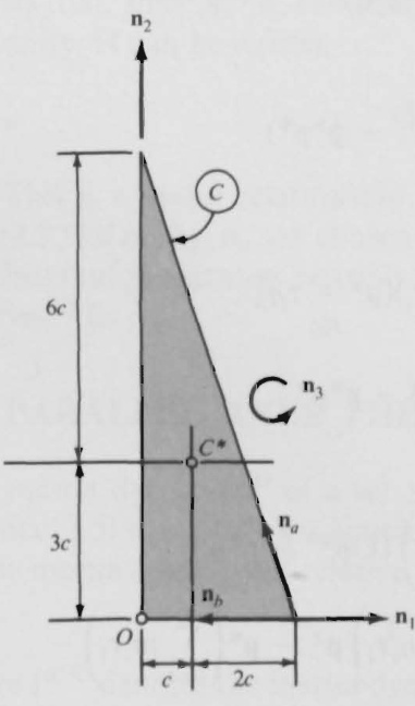
Figure 3.6.1

The position vector \pmb{\mathsf{p}} from _o to c^{*} is

\mathbf{p}^{*}=c\mathbf{n}_{1}+3c\mathbf{n}_{2}

Consequently, the product of inertia of a particle of mass \pmb{m} situated at c^{*} relative to ^o ,for \mathbb{n}_{a} and \mathbb{n}_{b} , is

I_{a b}^{\;\;C^{*}/\;O}\;=\;\;m({\bf p}^{*}\,\times\,{\bf n}_{a})\cdot({\bf p}^{*}\,\times\,{\bf n}_{b})\;\;=\;\;\frac{18m c^{2}}{(12,15)}\;\overline{{{\sqrt{10}}}}

and

I_{a b}^{\mathrm{\tiny~\it~c/0}}=I_{a b}^{\mathrm{\tiny~\itc/C^{*}}}+I_{a b}^{\mathrm{\tiny~\itc^{*}/O}}=\frac{81m c^{2}}{4\sqrt{10}}

3.7 EVALUATION OF INERTIA SCALARS

Generally speaking, the most direct way to find inertia scalars (see Sec. 3.3) of a set of particles (including sets consisting of a single particle) is to use Eq. (3.3.3). Exceptions to this rule arise when the value of an appropriate central inertia scalar (see Sec. 3.6) is known, in which event one can appeal to Eq. (3.6.4), or when a suitable inertia vector (see Sec. 3.3), inertia matrix, or inertia dyadic (see Sec. 3.5) is available, making it possible to use Eqs. (3.3.2), (3.5.3), or (3.5.20). In a sense, the opposite applies to the evaluation of inertia scalars of a body modeled as matter distributed along a curve, over a surface, or throughout a solid. Here, one should use Eq. (3.3.9), which is analogous to Eq. (3.3.3), only when one cannot find any tabulated information regarding the inertia properties of the body under consid. eration, which is likely to be the case only when the body has a variable mass densityrccupies an rregula igureWhen,as hapensmoreofteninenginering practice, the mass density is uniform and the figure in question is one of those considered nanavailable tableofinertia properties,thbest wayto procd istuse, frst, Eq. (3.4.3), (3.5.3), or (3.5.20) with I_{j k} ~~j,~k=1,2,3; representing central inertia scalars, and then to turn to Eq. (3.6.4), evaluating the last term in this equation with the aid of Eq. (3.3.3) after setting \nu=1 and m_{1} equal to the mass of the body. Appendix I contains information making it possibie to proceed in this way in connection with a number of figures chosen from among those encountered most frequently in enginering practice.

When an object can be regarded as composed of bodies B_{1},\dots,B_{v} , and an inertiacalrf thsbtwithrespttint \pmb{P} is to be found, one can use theaboveproceduretondthecorrespndinertiasalarfacf B_{1},\ldots,B_{v} with respect to \pmb{P}, and then simplyaddthese inertia scalarsThis fllows fromq. (333) and the assciativity of scalar adition.

Differentials sometimes can be used to advantage in connection with inertia calculations involving objects that can be regarded as thin-walled counterparts ofbdinwinsexad container c having sides of length \pmb{L} and let \pmb{k} be the radius o gyration of c with respect to a line passing through C^{*} , the mass center of c , and parallel to an edge of c Suppose, further, that the walls of c are thin. To determine \pmb{k} , let \rho be the mass density of a uniform solid cube S having sides of length L Then m , the mass of S, and \pmb{I} , the moment of inertia of \boldsymbol{s} about a line parallel to an edge of s and passing through s^{*} , the mass center of {\boldsymbol{s}} , are given by (see Appendix I)

m=\rho L^{3}

and

I={\frac{\rho L^{s}}{6}}

respectively, and the differentials of m and \boldsymbol{\mathit{I}} are

d m=3\rho L^{2}\,d L

and

d I={\frac{5\rho L^{4}}{6}}\,d L

Consequently, attributing to c the wall thickness d L/2 , and hence the mass dm and the moment of inertia \pmb{d I} , one can write

\frac{5\rho L^{4}}{6}\,d L_{_{(3.3.6)}}=\mathop{3\rho L^{2}}_{(3)}\,d L k^{2}

from which it follows immediately that

k=\frac{1}{3}\sqrt{\frac{5}{2}}\,L

The same result is obtained with somewhat more effort, but quite revealingly, by reasoning as follows

When c is regarded as formed by removing from a solid cube {\pmb S}_{1} of mass density \rho and having sides of length L_{1} a solid cube s_{2} of the same mass density and having sides of length L_{2} , the mass m and moment of inertia \pmb{I} d c about a line passing through C^{*} and parallel to an edge of c can be expressed as

m=\rho L_{1}{}^{3}-\rho L_{2}{}^{3}=\rho(L_{1}{}^{3}-L_{2}{}^{3})

and

I=\rho\frac{{L_{1}}^{5}}{6}-\rho\,\frac{{L_{2}}^{5}}{6}=\frac{\rho}{6}({L_{1}}^{5}-{L_{2}}^{5})

Consequently, \pmb{\bar{k}}, the radius of gyration of interest, is given by

\bar{k}\ {\underset{(3.3.6)}{=}}\left(\frac{I}{m}\right)^{1/2}\ {\underset{(7,8)}{=}}\left[\frac{{L_{1}}^{5}-{L_{2}}^{5}}{6({L_{1}}^{3}-{L_{2}}^{3})}\right]^{1/2}

Furthermore, in order for c to have sides of length \pmb{L} and walls of thickness t/2 L_{1} and L_{2} must be given by

L_{1}=L\;\;\;\;\;\;L_{2}=L-t

which leads to

\begin{array}{r l r}{\lefteqn{\bar{k}_{\ z,\left(9,10\right)}\frac{1}{\sqrt{6}}\bigg[\frac{L^{5}-\left(L-t\right)^{5}}{L^{3}-\left(L-t\right)^{3}}\bigg]^{1/2}}}\\ &{=}&{\frac{1}{\sqrt{6}}\left(\frac{5L^{4}-10L^{3}t+10L^{2}t^{2}-5L t^{3}+t^{4}}{3L^{2}-3L t+t^{2}}\right)^{1/2}}\end{array}

and

\operatorname*{lim}_{t\rightarrow0}\bar{k}=\frac{1}{3}\sqrt{\frac{5}{2}}L

Example The radius of gyration \pmb{k} of the body \pmb{B} described in the example in Sec. 3.2 and shown in Fig. 3.2.1 is to be found with respect to a line that is parallel to X_{2} and passes through B^{*} , the mass center of \boldsymbol{B}

Regarding \pmb{B} as composed of the three bodies B_{1},\;B_{2},\;B_{3} introduced previously, and noting that the masses of B_{1},B_{2},B_{3} are [see Eqs. (3.2.3)]

m_{1}=m\qquad m_{2}={\binom{\pi}{2}}m\qquad m_{3}=10\bigg(1+{\frac{\pi}{2}}\bigg)m

while \mathsf{\pmb{p}}^{\star} , the position vector from E to B^{*} , is given by

\mathbf{p}_{\textbf{\tiny=}_{(3.2.4)}}^{*}(1.82\mathbf{a}_{1}\,+\,2.03\mathbf{a}_{2}\,+\,0.318\mathbf{a}_{3})L

and the mass centers of B_{1},\,B_{2},\,B_{3} are the points B_{1}{}^{*},\,B_{2}{}^{*},\,B_{3}{}^{*} shown in Fig. 3.2.2, begin by forming expressions for the moment of inertia of \pmb{B}_{i} with respect to a line passing through B_{i}{}^{*}\,(i=1,2,3) and parallel to {\mathfrak{a}}_{2}

For B_{1} , from Eqs. (13), Fig. 3.2.2, and Appendix I,

{I_{2}}^{B_{1}/B_{1}}\mathbf{\Sigma}={\frac{m(6L)^{2}}{12}}=3m L^{2}

To deal with B_{2} , introduce unit vectors \mathbb{n}_{a} and \mathbb{n}_{b} as shown in Fig. 3.2.2, and refer to Appendix I to write

I_{a}^{~B_{2}/B_{2}^{*}}=\frac{(\pi/2)m(6L)^{2}}{2}\left[1+\frac{1}{\pi/2}-\frac{1}{(\pi/4)^{2}}\right]=0.438m L^{2}

I_{b}^{~~B_{2}/B_{2}*}=\frac{(\pi/2)m(6L)^{2}}{2}\left(1~-~\frac{1}{\pi/2}\right)=10.3m L^{2}

and then appeal to Eq. (3.4.3) to obtain

I_{2}^{~~B_{2}/B_{2}^{*}}=\biggl(\frac{1}{\sqrt{2}}\biggr)^{2}I_{a}^{~B_{2}/B_{2}^{*}}+\biggl(\frac{1}{\sqrt{2}}\biggr)^{2}\:I_{b}^{~B_{2}/B_{2}^{*}}{}_{(16,17)}^{*}\:5.36m L^{2}

Finally, refer to Appendix I to verify that

I_{2}^{\ B_{3}/B_{3}^{\star}}=10\bigg(1+\frac{\pi}{2}\bigg)m\,\frac{(6L)^{2}}{18}=51.4m L^{2}

Next, determine IB*/B* (i = 1, 2, 3) by using Eq. (3.3.3) with v = 1, that is, by expressing I_{2}^{\;\;B_{i}^{\star}/B^{\star}} as

I_{2}^{\phantom{}_{B_{i}}\star;|B^{\star}|}=\,m_{i}[({\bf p}^{*}-{\bf p}_{i})\,\times\,{\bf a}_{2}]^{2}\qquad(i=1,2,3)

where \pmb{{\mathsf{p}}_{i}} is the position vector from {\pmb E} (see Fig. 3.2.2) to B_{i}{}^{*}\;(i=1,2,3) Specifically,

\begin{array}{c}{{I_{2}^{{B_{1}}\ast\beta^{\ast}}=\displaystyle m[({\bf p}^{\ast}-3L{\bf a}_{3})\times{\bf a}_{2}]^{2}}}\\ {{\displaystyle(20)}}\\ {{\displaystyle=\,m L^{2}(1.82{\bf a}_{3}+2.68{\bf a}_{1})^{2}=10.5m L^{2}}}\\ {{\displaystyle(14)}}\\ {{\displaystyle I_{2}^{{B_{2}}\ast\beta^{\ast}}=\ \left(\frac{\pi}{2}\right)m\left\{\left[{\bf p}^{\ast}-\left(\frac{12L}{\pi}\right)({\bf a}_{2}+{\bf a}_{3})\right]\times{\bf a}_{2}\right\}^{2}\ =\ 24.5m L^{2}}}\\ {{\displaystyle(20)\left(\frac{1}{2}\right)m\left\{\left[({\bf p}^{\ast}-2L({\bf a}_{1}+{\bf a}_{2})\right]\times{\bf a}_{2}\right\}^{2}\ =\ 3.43m L^{2}}}\\ {{\displaystyle I_{2}^{{B_{3}}\ast\beta^{\ast}}=\ 10\ \left(1+\frac{\pi}{2}\right)m\left\{\left[({\bf p}^{\ast}-2L({\bf a}_{1}+{\bf a}_{2})\right]\times{\bf a}_{2}\right\}^{2}\ =\ 3.43m L^{2}}}\end{array}

Now refer to Eq. (3.6.5) to evaluate I_{2}^{{B_{i}}/{B^{*}}}\,(i=1,2,3) as

I_{2}{}^{B_{i}/B^{\star}}=I_{2}{}^{B_{i}/B_{i}}{}^{\star}+I_{2}{}^{B_{i}\star}/B^{\star}\qquad(i=1,2,3)

which gives

\begin{array}{l}{{I_{2}{}^{B_{1}/B^{\star}}=\;3m L^{2}+\;10.5m L^{2}=\;13.5m L^{2}\;}}\\ {{\phantom{I_{2}{}^{B_{1}/B^{\star}}=\;5.36m L^{2}+\;24.5m L^{2}=\;29.9m L^{2}\;}}}\\ {{\phantom{I_{2}{}^{B_{1}/B^{\star}}=\;51.4m L^{2}+\;3.43m L^{2}=\;54.8m L^{2}\;}}}\end{array}

Consequently,

I_{2}^{~~B/B^{*}}=I_{2}^{~^{B_{1}/B^{*}}}+I_{2}^{~^{B_{2}/B^{*}}}+I_{2}^{~^{B_{3}/B^{*}}}{}_{(2\,^{5}-2\,^{7})}^{}\,98.2m L^{2}

and

k\underset{(3.3.6)}{=}\left(\frac{I_{2}^{\;\;B/B^{\star}}}{m_{1}\,+\,m_{2}\,+\,m_{3}}\right)^{1/2}\underset{(13,28)}{=}1.86L

3.8 PRINCIPAL MOMENTS OF INERTIA

In general, the inertia vector {\mathbf{I}}_{\pmb{a}} (see Sec. 3.3) is not parallel to \mathbb{n}_{\pmb{a}} . When \pmb{\mathrm{\scriptscriptstyle{n}}}_{\pmb{\mathrm{\scriptscriptstyle{z}}}} is a unit vector such that \mathbf{I}_{z} is parallel to \pmb{\mathrm{\scriptscriptstyle{R}}}_{\pmb{\mathrm{\scriptscriptstyle{z}}}} , the line L_{z} passing through ^o and parallel to \pmb{\mathrm{\scriptscriptstyle{n}}}_{\pmb{\mathrm{\scriptscriptstyle{z}}}} is called a principal axis of \boldsymbol{s} for ^o , the plane P_{z} passing through ^o and normal to \pmb{\mathrm{\scriptscriptstyle{u}}}_{\pmb{\ z}} is called a principal plane of \boldsymbol{s} for ^o , the moment of inertia I_{z} of S with respect to L_{z} is called a principal moment of inertia of S for o , and the radius of gyration of S with respect to L_{z} is called a principal radius of gyration of S for o When the point ^o under consideration is the mass center of \pmb{S}, one speaks of central principal axes, central principal planes, central principal moments of inertia, and central principal radii of gyration.

When \mathbf{n_{z}} is parallel to a principal axis of \pmb{s} for ^o , the inertia vector \mathbf{I}_{z} of s relative to o for \pmb{\mathrm{\scriptscriptstyleR}}_{\pmb{\ z}} can be expressed as

\begin{array}{r}{\bar{\mathbf{I}}_{z}=I_{z}\bar{\mathbf{n}}_{z}}\end{array}

and, if \mathbf{n_{y}} is any unit vector perpendicular to \pmb{\mathrm{\scriptscriptstyle{u}}}_{\pmb{\ z}} , then the product of inertia of s relative to ^o for \mathbf{n_{y}} and \pmb{\mathrm{\scriptscriptstyle\equiv}}_{\pmb{\mathrm{\scriptscriptstyleZ}}} vanishes; that is,

I_{y z}=0

Suppose that \tilde{\mathbf{n}}_{1},\tilde{\mathbf{n}}_{2},\tilde{\mathbf{n}}_{3} are mutually perpendicular unit vectors, each parallel to a principal axis of \boldsymbol{s} for o and \mathbb{n}_{\pmb{a}} and \mathbb{n}_{b} are any two unit vectors. Then, if \pmb{a}_{i} and b; are defined as

a_{i}\triangleq\bar{\mathbf{n}}_{a}\cdot\bar{\mathbf{n}}_{i}\qquad b_{i}\triangleq\bar{\mathbf{n}}_{b}\cdot\bar{\mathbf{n}}_{i}\qquad(i=1,2,3)

the inertia scalar \pmb{I_{a b}} d \pmb{s} relative to ^o for \Biggl\triangledown_{\pmb{a}} and \bigtriangledown_{b} is given by

I_{a b}=a_{1}I_{1}b_{1}+a_{2}I_{2}b_{2}+a_{3}I_{3}b_{3}

where I_{1},I_{2},I_{3} are the principal moments of inertia of \pmb{s} for _o associated with n1, \mathfrak{n}_{2} ，， \mathbb{n}_{3} , respectively. This relationship is considerably simpler than its more general counterpart, Eq. (3.4.3), which applies even when \bar{\mathbf{n}}_{1},\bar{\mathbf{n}}_{2},\bar{\mathbf{n}}_{3} are not parallel to principal axes of \pmb{s} for o Similarly, Eqs. (3.5.1) and (3.522) reduce to

I=\left[{\begin{array}{c c c}{I_{1}}&{0}&{0}\\ {0}&{I_{2}}&{0}\\ {0}&{0}&{I_{3}}\end{array}}\right]

and

\mathbf{I}=I_{1}\mathbf{n}_{1}\mathbf{n}_{1}+I_{2}\,\mathbf{n}_{2}\,\mathbf{n}_{2}\,+I_{3}\,\mathbf{n}_{3}\,\mathbf{n}_{3}

respectively, when \mathbf{n}_{1},\mathbf{n}_{2},\mathbf{n}_{3} are parall toprincipal axesoffr ^o

For every set of particles there exists at least one set of three mutually perpendicular principal axes for everypoint in spaceTolocate principal axes of a set S of particlesfor a point ^o and to determine the associated principal moments of inertia, one exploits the following fcts.

\mathbf{n}_{1},\mathbf{n}_{2},\mathbf{n}_{3} are any mutually perpendicular unit vectors, I_{j k}\left(j,k=1,2,3\right) are the associated inertia scalars of \pmb{s} for ^o , and I_{z} is a principal moment of inertia of \pmb{s} for ^o , then I_{z} satisfies the cubic characteristic equation

\left|\begin{array}{c c c}{{(I_{1}\mathrm{~-~}I_{z})}}&{{I_{12}}}&{{I_{13}}}\\ {{I_{21}}}&{{(I_{2}\mathrm{~-~}I_{z})}}&{{I_{23}}}\\ {{I_{31}}}&{{I_{32}}}&{{(I_{3}\mathrm{~-~}I_{z})}}\end{array}\right|=0

A unit vector \bar{\mathbf{u}}_{\pmb{z}} is parallel to the principal axis associated with the principal moment of inertia I_{z} if

{\bf n}_{z}=z_{1}{\bf n}_{1}+z_{2}\,{\bf n}_{2}+z_{3}\,{\bf n}_{3}

where z_{1},z_{2},z_{3} satisfy the four equations

\sum_{j=1}^{3}z_{j}I_{j k}=I_{z}z_{k}~~~~~~(k=1,2,3)

{z_{1}}^{2}+{z_{2}}^{2}+{z_{3}}^{2}=1

When Eq. (7) has precisely two equal roots, every line passing through ^o and lying in the principal plane of \pmb{s} for ^o corresponding to the remaining root of Eq. (7) is a principal axis of S for ^o ; when Eq. (7) has three equal roots, every line passing through ^o is a principal axis of S for ^o

Once a principal plane \boldsymbol{P_{z}} of \pmb{s} for ^o has been identified, principal axes of S for ^o lying in \pmb{P_{z}} , as well as the associated principal moments of inertia of S for ^o can be found without solving a cubic equation. If \pmb{\mathrm{\scriptscriptstylem}}_{\pmb{\mathscr{a}}} and \mathbb{n}_{b} are any two unit vectors parallel to \boldsymbol{P_{z}} and perpendicular to each other, while \pmb{I_{a}},\pmb{I_{b}} , and \boldsymbol{I}_{a b} are the associated moments of inertia and product of inertia of S for ^o , then the angle \theta between \mathbb{n}_{\pmb{a}} and each of the principal axes in question satisfies the equation

\tan2\theta=\frac{2I_{a b}}{I_{a}-I_{b}}\qquad(I_{a}\ne I_{b})

and the associated principal moments of inertia of S for ^o say, \pmb{I_{x}} and I_{y} ,aregiven by

I_{x},I_{y}=\frac{I_{a}+I_{b}}{2}\pm\left[\left(\frac{I_{a}-I_{b}}{2}\right)^{2}+{I_{a b}}^{2}\right]^{1/2}

If I_{a}=I_{b} , then every line passing through o and lying in \pmb{P_{z}} is a principal axis of \pmb{S} for ^o , and the associated principal moments of inertia of \boldsymbol{s} for ^o all have the value I_{a}

Frequently, principal planes can be located by means of symmetry considerations. For example, when all particles of S lie in a plane, then this plane is a principal plane of S for every point of the plane, for the inertia vector of S relative to any point of the plane is then normal to the plane.

The eigenvalues of the matrix I defined in Eq. (3.5.1) are principal moments of inertia ofS for ^o because these eigenvalues satisfy Eq. (7); and, if a matrix [e_{1}\ e_{2}\ e_{3}] is an eigenvector of \pmb{I}, and {e_{1}}^{2}+{e_{2}}^{2}+{e_{3}}^{2}=1 then e_{1}\mathbf{n}_{1}+e_{2}\mathbf{n}_{2}+e_{3}\mathbf{n}_{3} is a unit vector parallel to a principal axis of \boldsymbol{s} for _o because \boldsymbol{e}_{1},\,\boldsymbol{e}_{2},\,\boldsymbol{e}_{3} then satisfy Eqs. (9) whenever I_{z} is an eigenvalue of I Hence, when computer routines for finding eigenvalues and eigenvectors of a symmetric matrix are available, these can be used directly to determine principal moments of inertia and to locate the associated principal axes.

Derivations When \pmb{\mathrm{\scriptscriptstyle{R}}}_{\pmb{\ z}} is parallel to a principal axis of s for o , and hence \mathbf{I}_{z} is parallel to \pmb{\mathrm{\scriptscriptstyle{u}}}_{\pmb{\ z}} , then there exists a quantity \lambda such that

\lambda\mathbf{n}_{z}=\mathbf{I}_{z}

Dot-multiplication of this equation with \pmb{\mathrm{\scriptscriptstyle{n}}}_{\pmb{\ z}} gives

\lambda=\mathrm{I}_{z}\cdot\mathrm{n}_{z}\underset{(3.3.2)}{=}I_{z}

and substitution from this equation into Eq. (13) yields Eq. (1). Furthermore, if \mathbf{n_{y}} is any unit vector perpendicular to \pmb{\mathrm{n}}_{\pmb{z}} , then dot-multiplication of Eq. (1) with \mathbf{n_{y}} and use of Eqs. (3.3.2) and (3.3.4) leads to Eq. (2).

If \mathbf{n}_{1},\,\mathbf{n}_{2},\,\mathbf{n}_{3} are mutually perpendicular unit vectors, each parallel to a principal axis of \boldsymbol{s} for ^o , then, in accordance with Eq. (2),

I_{12}=I_{23}=I_{31}=0

and substitution from these equations into Eqs. (3.4.3), (3.5.1), and (3.5.22) establishes the validity of Eqs. (4),(5), and (6), respectively.

\mathbf{If}\ \mathbf{n}_{1},\mathbf{n}_{2},\mathbf{n}_{3} are any mutually perpendicular unit vectors, I_{j k}(j,k=1,2,3) are theassociatednertia scalarf \pmb{s} for O,\,\mathfrak{n}_{\mathfrak{z}} is any unit vector, and z_{1},\,z_{2},\,z_{3} are defined as

z_{i}\triangleq\mathbf{n}_{z}\cdot\mathbf{n}_{i}\qquad(i=1,2,3)

then

\bar{\mathbf{n}}_{z}\mathop{=}_{(1.3,1)}\sum_{k\mathop{=}1}^{3}z_{k}\mathbf{n}_{k}

and

\mathbf{I}_{z}\underset{(3,4,1)}{=}\sum_{j=1}^{3}z_{j}\mathbf{I}_{j}

Now

\mathbf{I}_{j}=\sum_{(1,3,3)}^{3}\,\mathbf{I}_{k}=\mathbf{n}_{k}\,\mathbf{n}_{k}\,\mathbf{\phi}_{(3,3,2)}^{=}\sum_{k=1}^{3}I_{j k}\,\mathbf{n}_{k}\qquad(j=1,2,3)

Hence,

\mathbf{I}_{z}\underset{(18,19)}{=}\sum_{j=1}^{3}\sum_{k=1}^{3}z_{j}I_{j k}\mathbf{n}_{k}

and \pmb{\mathrm{\scriptscriptstylem}}_{\pmb{z}} is parallel to a principal axis of \boldsymbol{s} for o if

\sum_{j=1}^{3}\sum_{k=1}^{3}z_{j}I_{j k}\mathfrak{n}_{k}=I_{z}\sum_{k=1}^{3}z_{k}\mathfrak{n}_{k}

This vector equation is equivalent to the three scalar equations

\sum_{j=1}^{3}z_{j}I_{j k}=I_{z}z_{k}~~~~~~(k=1,2,3)

Also, z_{1},z_{2},z_{3} satisfy the equation

{z_{1}}^{2}\mathrm{~+~}{z_{2}}^{2}\mathrm{~+~}{z_{3}}^{2}\mathrm{~=~}1

because \pmb{\mathrm{\scriptscriptstylem}}_{\pmb{\ z}} is a unit vector. [Equations (22) and (23) are Eqs. (9) and (10), respectively.] As Eqs. (22) are linear and homogeneous in z_{1},z_{2},z_{3} , and as these three quantities cannot all vanish, for this would violate Eq. (23), Eqs. (22) can be satisfied only if the determinant of the coefficients of z_{1},\,z_{2},\,z_{3} vanishes, that is, if Eq. (7) is satisfied. Now, Eq. (7) is cubic in I_{z} . Hence, there exist three values of I_{z} (not necessarily distinct) that satisfy Eq. (7). It will now be shown that all such values of I_{z} are real.

Let A,B,\alpha_{j} , and \beta_{j}\,(j=1,2,3) be real quantities such that

I_{z}=A\,+\,i B

and

z_{j}=\alpha_{j}+i\beta_{j}\qquad(j=1,2,3)

where i\triangleq\sqrt{-1} .Then

\sum_{j=1}^{3}\;(\alpha_{j}\:+\:i\beta_{j})I_{j k}\underset{(22)}{=}(A\:+\:i B)(\alpha_{k}\:+\:i\beta_{k})\qquad(k\:=\:1,\:2,\:3)

and, after separating the real and imaginary parts of this equation, one has

\begin{array}{l l}{{{\displaystyle\sum_{j=1}^{3}\alpha_{j}I_{j k}\,=\,A\alpha_{k}\,-\,B\beta_{k}~~}}}&{{(k=1,2,3)}}\\ {{{}}}&{{{}}}\\ {{{\displaystyle\sum_{j=1}^{3}\beta_{j}I_{j k}\,=\,B\alpha_{k}\,+\,A\beta_{k}~~}}}&{{(k=1,2,3)}}\end{array}

Multiply Eq. (28) by \pmb{\alpha_{k}} and Eq. (27) by \beta_{\pmb{k}} , and subtract, obtaining

\sum_{j=1}^{3}\alpha_{k}\beta_{j}I_{j k}-\sum_{j=1}^{3}\alpha_{j}\beta_{k}I_{j k}=B({\alpha_{k}}^{2}+\,\beta_{k}{}^{2})\qquad(k\,=\,1,\,2,\,3)

and add these three equations, which yields

\sum_{k=1}^{3}\sum_{j=1}^{3}\,\alpha_{k}\beta_{j}I_{j k}\,-\,\sum_{k=1}^{3}\sum_{j=1}^{3}\,\alpha_{j}\beta_{k}I_{j k}\,=\,B\sum_{k\,=\,1}^{3}\,({\alpha_{k}}^{2}\,+\,{\beta_{k}}^{2})\;

Now,

\sum_{k=1}^{3}\sum_{j=1}^{3}\,\alpha_{k}\beta_{j}I_{j k}\equiv\sum_{k=1}^{3}\sum_{j=1}^{3}\alpha_{j}\beta_{k}I_{k j}\mathop{=}_{(3.3.4)}\sum_{k=1}^{3}\sum_{j=1}^{3}\,\alpha_{j}\beta_{k}I_{j k}

Consequently, the left-hand member of Eq. (30) is equal to zero, and Eq. (30) reducesto

B\sum_{k=1}^{3}\,({\alpha_{k}}^{2}\,+\,{\beta_{k}}^{2})\,=\,0

The quantities \pmb{\alpha_{k}} and \beta_{k}\,(k=1,2,3) cannot all vanish, for this would mean [see Eqs. (25)] that z_{1},z_{2},z_{3} all vanish, which is ruled out by Eq. (23). Hence, the only way Eq. (32) can be satisfed is for \boldsymbol{B} to be equal to zero, and Eq. (24) thus shows that I_{z} is real.

Suppose that two roots of Eq. (7), say, I_{x} and I_{y} , are distinct from each other. Then, with self-explanatory notation, we can write

\begin{array}{r}{\mathbf{I}_{x}=I_{x}\mathbf{n}_{x}}\\ {\mathbf{\eta}_{(1)}^{(1)}}\\ {\mathbf{I}_{y}=I_{y}\mathbf{n}_{y}}\\ {\mathbf{\eta}_{(1)}^{(1)}}\end{array}

whereupon dot-mutliplication of Eq. (33) with \mathbf{n_{y}} , Eq. (34) with \bar{\mathbf{n}}_{z} , and subtraction of the resulting equations produces

\mathbf{I}_{x}\cdot\mathbf{n}_{y}\,-\,\mathbf{I}_{y}\cdot\mathbf{n}_{x}=(I_{x}\,-\,I_{y})\mathbf{n}_{x}\cdot\mathbf{n}_{y}

or, in view of Eq. (3.3.2)

I_{x y}-I_{y x}\underset{(3.3.4)}{=}0\,=\,(I_{x}-I_{y})\mathfrak{n}_{x}\cdot\mathfrak{n}_{y}

Since I_{x} differs from I_{\mathrm{y}} by hypothesis it follows that

\mathbf{n}_{\mathbf{x}}\cdot\mathbf{n}_{\mathbf{y}}=0

which proves that, whenever two principal moments of inertia of S for o are unequal, the corresponding principal axes of s for ^o are perpendicular to each other. Consequently, when Eq. (7) has three distinct roots, a unique principal axis of S for o corresponds to each root, and these three principal axes of S for o are mutually perpendicular. What remains to be done, is to deal with the matter of repeated roots of Eq. (7).

Let I_{c} denote one of the roots of Eq. (7), let \mathbf{\Psi}_{\mathbf{c}} be a unit vector parallel to the asociated principal axisofSfor ^o and suppose that the remaining two roots of Eq.(7) are equal t each other(and possibly to I_{c} .Let \Biggl\triangledown_{\pmb{a}} and \mathbb{n}_{b} be any unit vectors perpendicular to \bar{\mathbf{n}}_{c} and to each other, and note that. in acordance with Eq. 2).

I_{a c}\underset{(3.3.4)}{=}I_{c a}=0\qquad I_{b c}\underset{(3.3.4)}{=}I_{c b}=0

In Eq. (7), the subscripts 1, 2, and 3 may be replaced with a,b and c ,respectively. When this is done and Eqs. (38) are used, Eq. (7) reduces to

(I_{c}-I_{z})[{I_{z}}^{2}-(I_{a}+I_{b})I_{z}+I_{a}I_{b}-{I_{a b}}^{2}]=0

which has the three roots

I_{z}=\frac{I_{a}+I_{b}}{2}\pm\bigg[\bigg(\frac{I_{a}-I_{b}}{2}\bigg)^{2}+I_{a b}^{~~2}\bigg]^{1/2},\qquad I_{c}

The first two of these can be equal to each other only if

\left(\frac{I_{a}-I_{b}}{2}\right)^{2}\,+\,I_{a b}^{\;\;\;2}=0

which is possible only if

I_{a}=I_{b}

and

I_{a b}=0

But Eqs. (40) shows that, under these circumstances, I_{a} is one of the values of I_{z} that is, I_{a} is a principal moment of inertia of S for o , and \mathbb{n}_{a} is thus parallel to a principal axis of S for o Since \Biggl\triangledown_{\pmb{a}} was restricted only to the extent of being required to be perpendicular to \scriptstyle\mathbf{\delta}\mathbf{n}_{c} , this means that every line passing through o and perpendicular to \mathbf{u}_{c} is a principal axis of s for o ; it follows from this that, when Eq. (7) has three equal roots, every line passing through o is a principal axis of S for o

The validity of Eqs. (12) is established by Eqs. (40). Finally, Eq. (11) may be derived from Eqs. (9) by writing the first of these with the subscripts 1, 2, and 3 replaced with a,b, and c , respectively, and with I_{c a} set equal to zero in accordance with Eqs. (38), which gives

z_{a}I_{a}+\,z_{b}I_{a b}=I_{z}z_{a}

where z_{a} and z_{b} are then the \Biggl\triangledown_{a} and \mathbf{n}_{b} measure numbers of a unit vector \mathbf{n}_{z} that is parallel to one of the principal axes of s for o associated with the first two values of I_{z} in Eqs. (40). The unit vectors \mathbf{n}_{a},\,\mathbf{n}_{b} . and \bar{\mathbf{n}}_{z} are shown in Fig. 3.8.1, as is the angle \theta ,which is seen to satisfy the equation

\tan\theta={\frac{z_{b}}{z_{a}}}

Now,

\tan2\theta={\frac{2\tan\theta}{1\,-\tan^{2}\theta}}_{(45)}={\frac{2(z_{b}/z_{a})}{1\,-\,(z_{b}/z_{a})^{2}}}

and

{\frac{z_{b}}{z_{a}}}={\frac{I_{z}-I_{a}}{I_{a b}}}=\mathrm{\Omega}-{\frac{1}{I_{a b}}}\left\{{\frac{I_{a}-I_{b}}{2}}\pm\left[\left({\frac{I_{a}-I_{b}}{2}}\right)^{2}+{\cal I}_{a b}{}^{2}\right]^{1/2}\right\}

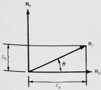
Figure 3.8.1

so that

1-\left(\frac{z_{b}}{z_{a}}\right)^{2}=\mathrm{~-~}\frac{I_{a}\mathrm{~-~}I_{b}}{{I_{a b}}^{2}}\left\{\frac{I_{a}\mathrm{~-~}I_{b}}{2}\pm\left[\left(\frac{I_{a}\mathrm{~-~}I_{b}}{2}\right)^{2}+{I_{a b}}^{2}\right]^{1/2}\right\}

Thus, Eq. (11) is obtained by substituting from Eqs. (47) and (48) into Eq. (46).

Example A uniform rectangular plate B of mass m has the dimensions shown in Fig. 3.8.2. Two sets of principal moments of inertia and associated principal axes of B are to be found, namely, the principal moments of inertia Ix, Iy, I of B for \upsilon and the associatedprincipalaxes X Y,Z ,andtheprincipalmoments ofinertia I_{x}^{\prime} I_{y}^{\prime} I_{z}^{\prime} of B for O^{\prime} and the associated principal axes X^{\prime} Y' Z^{\prime} where O^{\prime} is apoint situated at a distance 3L from o on a line passing through \upsilon and parallel to \mathbf{n}_{3} , as shown in Fig. 3.8.2, and \ensuremath{\mathbf{n}}_{3}=\ensuremath{\mathbf{n}}_{1}\times\ensuremath{\mathbf{n}}_{2}

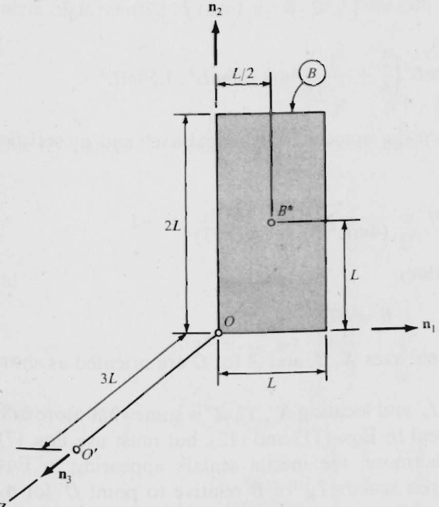
Figure 3.8.2

Table 3.8.1

<html>

Iik	一		3.
一	4mL2:3	-mL²2	0
2	-mL².2	mL².3	0
3	0	0	5mL²/3

</html>

When, as in the example in Sec. 3.3, B is modeled as matter distributed over a rectangular surface, this surface is a principal plane of B for o , the line Z passing through o and parallel to \mathfrak{n}_{3} is a principal axis of S for o , and the corresponding principal moment of inertia of B for O,\;I_{z} , is equal to the moment of inertia of B about Z . Referring to Table 3.8.1, where the inertia scalars I_{j k} of B relative to o for \bar{\mathbf{n}}_{j} and {\bf n}_{k}\left(j,k=1,2,3\right) I are recorded in accordance with Table 3.4.1, one thus finds that

I_{z}=I_{33}={\frac{5m L^{2}}{3}}=1.67m L^{2}

and the remaining principal moments of inertia of B for O,I_{x} and I_{y} , found with the aid of Eq. (12), where the subscripts ^{a} and ^b may be replaced with 1 and 2, respectively, are given by

\begin{array}{c}{{I_{x},\,I_{y}=\displaystyle\frac{5m L^{2}}{6}\pm\left[\left(\displaystyle\frac{m L^{2}}{2}\right)^{2}+\left(\displaystyle\frac{m L^{2}}{2}\right)^{2}\right]^{1/2}}}\\ {{=m L^{2}\displaystyle\left(\frac{5}{6}\pm\displaystyle\frac{1}{\sqrt{2}}\right)=0.126m L^{2},\,1.54m L^{2}}}\end{array}

while the angle \boldsymbol{\theta} between the associated principal axes and \mathbf{n}_{1} satisfies the equation

\tan2\theta\,=\,{\frac{-2(m L^{2}/2)}{(11)}}{\overline{{(4m L^{2}/3)}}}{\overline{{-(m L^{2}/3)}}}=\,-\,1

so that \theta can have the values

\theta=67.5^{\circ},-22.5^{\circ}

Consequently, the principal axes X,\,Y, and Z for o are oriented as shown in Fig. 3.8.3.

Determining I_{x}^{\;\;^{\prime}},I_{y}^{\;\;^{\prime}},I_{z}^{\;\;^{\prime}} and locating X^{\prime},\,Y^{\prime},Z^{\prime} is somewhat more difficult, for here one cannot appeal to Eqs. (11) and (12), but must use Eqs. (7), (9). and (10), instead. Furthermore, the inertia scalars appearing in Eqs. (7) and (9) must be the inertia scalars I_{j k}{}^{'} of B relative to point O^{\prime} for \mathbf{n}_{j} and \mathtt{m}_{k}\left(j,k=1,2,3\right) . which are not, as yet, available. To find them, let I^{*} denote the inertia matrix of B relative to B^{*} the mass center of B for \mathbf{n}_{1} \mathbf{n}_{2},\mathbf{n}_{3} ,and refer to Eq. (3.6.2) to write

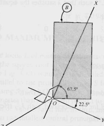
Figure 3.8.3

\begin{array}{r l}&{I^{*}\,=\,I\,-\,I^{B^{*}/O}}\\ &{I^{\prime}\,=\,I^{*}\,+\,I^{B^{*}/O^{\prime}}}\\ &{\phantom{I^{*}\,=\,}=\,I\,-\,I^{B^{*}/O}\,+\,I^{B^{*}/O}}\end{array}

where I^{\prime} is the inertia matrix of B relative to U for \mathbf{n}_{1},\,\mathbf{n}_{2},\,\mathbf{n}_{3} ,and I the inertia matrix of \boldsymbol{B} relative to \mathcal{O} for \boldsymbol{\Pi}_{1} \mathbf{u}_{2} n_{3} , then can be written (see Table 3.8.1)

I=m L^{2}{\left[\begin{array}{l l l}{{\frac{4}{3}}}&{-{\frac{1}{2}}}&{0}\\ {-{\frac{1}{2}}}&{{\frac{1}{3}}}&{0}\\ {0}&{0}&{{\frac{5}{3}}}\end{array}\right]}

while I^{B^{*}/O} and I^{B^{\kappa}/O^{\prime}} ,found with the aid of Eqs. (3.3.3), are given by

I^{B^{\star}/O}=m L^{2}\left[-{\frac{1}{2}}\begin{array}{r r r}{{1}}&{{-{\frac{1}{2}}}}&{{0}}\\ {{-{\frac{1}{2}}}}&{{{\frac{1}{4}}}}&{{0}}\\ {{0}}&{{0}}&{{{\frac{5}{4}}}}\end{array}\right]

and

I^{B^{\ast}/O^{\prime}}=m L^{2}\left[-{\frac{1}{2}}\quad{\frac{37}{4}}\quad\quad{\frac{3}{4}}\atop{3}\right]

Consequently,

\begin{array}{r}{I^{\prime}=\phantom{-}m L^{2}\left[-\frac{3}{2}\frac{1}{2}\right.\qquad\left.\frac{3}{2}\right.\qquad}\\ {\phantom{-}\!\!\!(54\!-\!57)\phantom{-}\!\!\!\!(\frac{3}{2}\!\!-\!\!\!\frac{1}{3}\!\!\!\!)\phantom{-}\!\!\!\!\frac{28}{3}\phantom{-}\!\!\!\!(\frac{5}{3}\!\!\!-\!\!\!\frac{1}{3}\!\!\!\!)}\end{array}

The eigenvalues of I^{\prime} are values of m L^{2}\lambda such that \lambda satisfies the equation

\begin{array}{r}{\left|\begin{array}{c c c c c}{31}&{-\lambda}&{}&{-\frac{1}{2}}&{}&{\frac{3}{2}}\\ {-\frac{1}{2}}&{}&{\frac{28}{3}-\lambda}&{}&{3}\\ {\frac{3}{2}}&{}&{3}&{}&{\frac{5}{3}-\lambda}\end{array}\right|_{(7,58)}=\ 0}\end{array}

which is the case for

\lambda=0.381131,10.3665,10.5857

Hence,

I_{x}^{\ \prime}=0.381131m L^{2}\qquad I_{y}^{\ \prime}=10.3665m L^{2}\qquad I_{z}^{\ \prime}=10.5857m L^{2}

To locate X^{\prime} , the principal axis of B for O^{\prime} associated with I_{x}^{\;\;\prime} , refer to Eqs. (9) to write

\begin{array}{r}{z_{1}I_{11}^{\ \prime}+z_{2}I_{21}^{\ \prime}+z_{3}I_{31}^{\ \prime}=I_{x}^{\ \prime}z_{1}}\\ {z_{1}I_{12}^{\ \prime}+z_{2}I_{22}^{\ \prime}+z_{3}I_{32}^{\ \prime}=I_{x}^{\ \prime}z_{2}}\end{array}

or, by reference to Eqs. (58) and (61).

\begin{array}{l}{{z_{1}(\frac{31}{3}-0.381131)\,+\,z_{2}(-\frac{1}{2})\,=\,z_{3}(-\frac{3}{2})}}\\ {{\ }}\\ {{z_{1}(-\frac{1}{2})\,+\,z_{2}(\frac{28}{3}-0.381131)\,=\,z_{3}(-3)}}\end{array}

Solution of these two equations for z_{1} and z_{2} yields

z_{1}=\,-0.1680z_{3}\qquad z_{2}=\,-0.3445z_{3}

and substitution into Eq. (10) shows that z_{3} must satisfy the equation

[(-0.1680)^{2}+(-0.3445)^{2}+1]z_{3}{}^{2}=1

which is satisfied by

z_{3}=\pm0.9338

Hence,

\begin{array}{r}{z_{1}\underset{(66,68)}{=}\mp0.1569\qquad z_{2}=\mp0.3217}\end{array}

and X' is parallel to the unit vector x' defined as

\begin{array}{r}{\mathbf{x}^{\prime}\triangleq\mp0.157\mathbf{n}_{1}\mp0.322\mathbf{n}_{2}\pm0.934\mathbf{n}_{3}}\\ {\mathbf{\Sigma}_{(69)}^{(69)}\quad\quad\quad\quad\quad\quad\quad\quad\quad}\end{array}

Similarly, to locate Y^{\prime} and Z^{\prime} , one needs only to replace 0.381131 with 10.3665 and 10.5857, respectively [see Eqs. (61)]. in Eqs. (64) and (65), solve the resulting equations for z_{1} and z_{2} in terms of z_{3} , and then use Eq. (10) to find that Y^{\prime} and Z^{\prime} are parallel to the unit vectors \mathbf{y}^{\prime} and \mathbf{z}^{\prime} defined as

\mathbf{y}^{\prime}\triangleq\mp0.0724\mathbf{n}_{1}\pm0.947\mathbf{n}_{2}\pm0.314\mathbf{n}_{3}

and

\mathbf{z}^{\prime}=\mp0.985\mathbf{n}_{1}\mp0.0185\mathbf{n}_{2}\mp0.172\mathbf{n}_{3}

3.9 MAXIMUM AND MINIMUM MOMENTS OF INERTIA

The locus E of points whose distance R from a point O is inversely proportional to the squarerootof themoment ofinertia of a set {\cal{S}} of particles about line o P （Fislall \boldsymbol{S} for {\cal O} whose axes are parallel to the principal axes o s for \upsilon (see Sec. 3.8). It fllows that, of all lines passing through o , those with respect to which s has aargerrmal of inertia thanit has withrespect to all other lines passing through O are principal axes of \boldsymbol{\mathrm{_{\Delta}}} for o and thisueans that mmentfit s is smaller than the smallet central principalmoment of inertia of \boldsymbol{s}

Derivations In Fig. 3.9.1, \boldsymbol{X} Y,Z designatemutuallyperpendicularcoordinate axes passing through o chosen in such a way that achis a principal axisf \boldsymbol{S} for o x z are the coordinates of P \mathbf{n}_{x} {\bf{I}}_{y} {\bf{n}}_{z} are unit vectors parallel to X Y. Z respectively; and \Pi_{a} is a unit vector parallel to O P It is to be shown that x satisfy the equation of an ellipsoid whenever

R=\lambda{{I_{a}}^{-1/2}}

Where I is th moment ofinertia of S with respect to line OP,and is anyconstant. Let

a_{x}\triangleq\mathbf{n}_{a}\cdot\mathbf{n}_{x}\quad\quad a_{y}\triangleq\mathbf{n}_{a}\cdot\mathbf{n}_{y}\quad\quad a_{z}\triangleq\mathbf{n}_{a}\cdot\mathbf{n}_{z}

So that

\mathbf{n}_{a}=a_{x}\mathbf{n}_{x}+a_{y}\mathbf{n}_{y}+a_{z}\mathbf{n}_{z}

and note that the position vector from O to P can be expressed both as Rng and as x\mathbf{n}_{x}+y\mathbf{n}_{y}+z\mathbf{n}_{z} so that, in view of Eq.(3),

a_{x}={\frac{x}{R}}\qquad a_{y}={\frac{y}{R}}\qquad a_{z}={\frac{z}{R}}

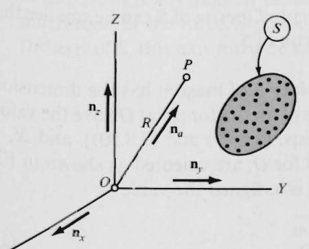
Also,

{I_{u}}\quad=\quad{a_{x}}^{2}I_{x}+{a_{y}}^{2}I_{y}+{a_{z}}^{2}I_{z}

where I_{x},I_{y},I_{z} are the principal moments of inertia of s for o . Hence,

I_{a\_}=\frac{1}{R^{2}}(x^{2}I_{x}+y^{2}I_{y}+z^{2}I_{z})

and elimination of R by reference to Eq. (1) leads to

{\frac{x^{2}}{x^{2}}}+{\frac{y^{2}}{\beta^{2}}}+{\frac{z^{2}}{\gamma^{2}}}=1

where x,\beta,\,\gamma are defined as

\varkappa\triangleq\lambda I_{s}^{\mathrm{~\,~-~}1/2}\qquad\beta\triangleq\lambda I_{\mathrm{y}}^{\mathrm{~\,~-~}1/2}\qquad\gamma\triangleq\lambda I_{z}^{\mathrm{~\,~-~}1/2}

Equation (7) is the equation of an ellipsoid whose axes are X,\,Y,\,Z. , that is, the principal axes of s for o . and whose semidiameters have lengths \mathfrak{x},\,\beta,\,\gamma given by Eqs. (8). Now, the naming of the axes always can be accomplished in such a way that I_{z}\geq I_{\mathrm{y}}\geq I_{x} or, in view of Eqs. (8), that \because\leq\beta\leq\alpha , and the distance \pmb R from the center o to any point P of an ellipsoid is never smaller than the smallest semidiameter, and never larger than the largest semidiameter, which then means that

\because\le R\le\alpha

Using Eqs. (1) and (8) to eliminate R,\,\mathfrak{x}. and \because gives

I_{z}^{\ -1/2}\leq I_{a}^{\ -1/2}\leq I_{x}^{\ -1/2}

or, equivalently,

I_{z}\geq I_{a}\geq I_{x}

which shows that the moment of inertia of s about a line that passes through o and is not a principal axis of s for o cannot be smaller than the smallest, or larger than the largest, principal moment of inertia of s for o . Finally, the moment of inertia of s about a line that does not pass through the mass center of s always exceeds the moment of inertia of s about a parallel line that does pass through the mass center [see Eq. (3.6.5)]. Hence, no moment of inertia of s can be smaller than the smallest central principal moment of inertia of S.

Example When a uniform rectangular plate B of mass m has the dimensions shown in Fig. 3.8.2, its principal moments of inertia for point o have the values 0.126m L^{2} ， 1.54m L^{2} , and 1.67m L^{2} [see Eqs. (3.8.49) and (3.8.50)], and X ,Y, and Z , the respective principal axes of B for o , are oriented as shown in Fig. 3.8.3. Hence, if the constant \lambda in Eqs. (8) is assigned the value

\lambda=\frac{L^{2}\sqrt{m}}{2}

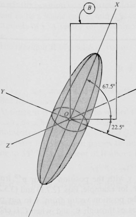
Figure 3.9.2

then the principal semidiameters of the associated inertia ellipsoid of B for O havelengths \boldsymbol{\alpha} \beta and \gamma given, in accordance with Eqs. (8), by

\alpha=\frac{L}{2\sqrt{0.126}}=1.4L\qquad\beta=0.40L\qquad\gamma=0.39L

and the ellipsoid appears as shown in Fig. 3.9.2. Furthermore, the moment of inertia of B about line X is smaller than themoment of inertia of \boldsymbol{B} about any other line passing through point \upsilon This fact is of practical interest in the following situation.Suppose that a shaft S is fixed in a reference frame A ,and it is desired to mount \boldsymbol{\mathbf{\mathit{\varepsilon}}}_{E} on S in such a way that the axis of \dot{S} passes through \boldsymbol{o} while the magnitude of a force applied to B normal to the plane of B in order to impart to B^{\prime} any angular acceleration in _A is as small as possible. Since the magnitude of the force is proportional to the moment of inertia of B about the axis of S,this axismust bemade to coincide with X

GENERALIZED FORCES

The necessity to cross-multiply a vector \mathbf{v} with the position vector {\mathfrak{p}}^{A B} from a point A to a point B arises frequently [see, for example, Eqs. (2.7.1) and (3.5.27)]. Now, {\bf p}^{A B}\mathrm{\bf~\times~}{\bf v}={\bf p}^{A C}\mathrm{\bf~\times~}{\bf v}, where \mathfrak{p}^{A C} is the position vector from A to any point C of the line L that is parallel to v and passes through B; and, when C is chosen properly, it may be easier to evaluate \mathsf{\pmb{p}}^{A C} x v than \boldsymbol{\mathsf{p}}^{A B}\,\times\,\boldsymbol{\mathsf{v}}. This fact provides the motivation for introducing the concepts of “bound" vectors and “moments" of such vectors as in Sec. 4.1. The terms “couple” and “torque,” which have to do with special sets of bound vectors, are defined in Sec. 4.2, and the concepts of "equivalence" and “replacement,” each of which involves two sets of bound vectors, are discussed in Sec. 4.3. This material then is used throughout the rest of the chapter to facilitate the forming of expressions for quantities that play a preeminent role in connection with dynamical equations of motion, namely, two kinds of generalized forces. Sections 4.4-4.10 deal with generalized active forces, which come into play whenever the particles of a system are subject to the actions of contact and/or distance forces. Generalized inertia forces, which depend on both the motion and the mass distribution of a system, are discussed in Sec. 4.11. Mastery of the material brings one into position to formulate dynamical equations for any system possessing a finite number of degrees of fredom, as may be ascertained by reading Sec. 6.1.

4.1 MOMENT ABOUT A POINT, BOUND VECTORS, RESULTANT

Of the infinitely many lines that are parallel to every vector v, a particular one, say，, L , called the line of action of v, must be selected before M, the moment of \mathbf{v} aboutapoint P , can be evaluated, for M is defined as

wherepis thepositionvector from P to any point on L Once L hasbeenspecified, \gamma is said to be a bound vector, and it is customary to show \mathbf{v} on L in pictorial representations of \gamma A vector for which no line of action is specified is called a free vector.

The resultant \mathbf{R} ofa set \boldsymbol{S} of vectors \mathbf{\nu}_{1},\dots,\mathbf{\nu}_{v} is defined as

\mathbb{R}\triangleq\sum_{i=1}^{\nu}\mathbb{v}_{i}

and,if \mathbf{v}_{1},\ldots,\mathbf{v}_{\nu} are bound vectors, the sum of their moments about a point P is called the moment of S about P.

At times, it is convenient to regard the resultant \mathbf{k} of a set {\cal{S}} of boundvectors \mathbf{\nu}_{1},\dots,\mathbf{v}_{\nu} as a bound vector. Suppose, for example, that \mathbf{M}^{\mathbf{s}/P} and {\bf{M}}^{s/Q} denote the moments of {\cal{S}} about points P and \mathcal{Q} respectivly, and \mathbf{R} isregarded as abound vector whose line of action passesthrough \boldsymbol{Q} . Then one can find {\bf M}^{{\bf S}/{P}} simply by adding to \mathbf{M}^{S/Q} themoment of Rabout P for

\mathbf{M}^{S/P}=\mathbf{M}^{S/Q}+\mathbf{r}^{P Q}\times\mathbf{R}

Where \mathbf{r}^{P Q} is the positionvector from P to \mathcal{Q}

DerivationLet and be the position vectors from P and \mathcal{Q} respetivly,to a \mathbf{p}_{i} {\bf q}_{i}
point on the line of action L_{i} of \mathbf{v}_{i}\,(i=1,\ldots,\nu) ,and let be the position vector
from P to \mathcal{Q} , as shown in Fig. 4.1.1. Then, by defnition,

\mathbf{M}^{s_{i},s_{i}}=\sum_{i=1}^{v}\mathbf{p}_{i}\times\mathbf{\omega}\mathbf{v}_{i}

and

\mathbf{M}^{S/Q}=\sum_{i=1}^{\nu}\mathbf{q}_{i}\times\mathbf{\omega}\mathbf{v}_{i}

Now (see Fig, 4.1.1),

\mathbf{p}_{i}=\mathbf{r}^{p_{Q}}+\mathbf{q}_{i}\qquad(i=1,\ldots,\nu)

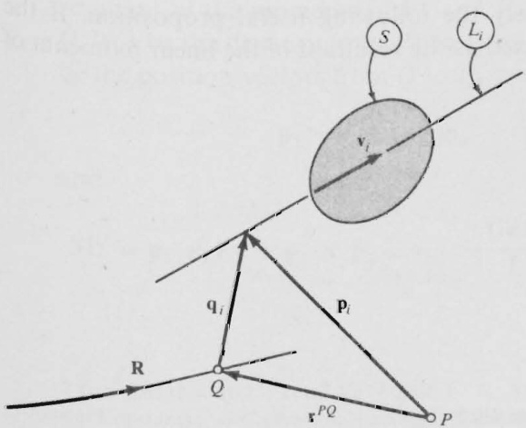
Figure 4.1.1

Hence,

\begin{array}{c}{{{\bf{M}}^{S/P}=\displaystyle\sum_{i=1}^{\nu}\,(\mathrm{{y}}^{P Q}+{\bf{q}}_{i})\times\mathrm{{\bf{v}}}_{i}=\mathrm{{\bf{r}}}^{P Q}\times\displaystyle\sum_{i=1}^{\nu}\mathrm{{\bf{v}}}_{i}+\sum_{i=1}^{\nu}\mathrm{{\bf{q}}}_{i}\times\mathrm{{\bf{v}}}_{i}}}\\ {{=\mathrm{{\bf{r}}}^{P Q}\times\mathrm{{\bf{{R}}}}+\mathrm{{\bf{M}}}^{S/Q}}}\end{array}

This establishes the validity of Eq.(3). If \mathbf{R} is regarded as a bound vector whose line of action passes through \boldsymbol{Q} , then, in accordance with Eq. (1), \mathfrak{r}^{P Q}\,\times\,\mathbb{R} isthe momentof \mathbf{R} about P

Exampie In Fig. 4.1.2, \displaystyle P and \mathcal{Q} are two points of a rigid body B that is moving in a reference frame A . If the angular velocity {}^{A}{\bf\omega}{\bf\omega}^{B} of B in A is regarded as a boundvector whose line of action passes through Q ,then M,the moment of {}^{A}\mathbf{\wp}^{B} about point P , is given by

\mathbf{M}=\mathbf{\Pi}-\mathbf{r}\times\mathbf{\Pi}^{A}\mathbf{\Theta}\mathbf{\Theta}^{B}

where \pmb{\Gamma} is the position vector from \boldsymbol{Q} to P ,as shown inFig.4.1.2.This moment vector is equal to the difference between the velocities of P and \mathcal{Q} in A ,for

\begin{array}{c}{\mathbf{M}={^{A}\mathbf{\omega}^{0}}{^{B}}\times\mathbf{r}\quad={^{A}\mathbf{v}^{P}}-{^{A}\mathbf{v}^{Q}}}\\ {{^{(8)}}}\end{array}

If S is a set of particles P_{1},\dots,P_{v} of masses m_{1},\ldots,m_{\nu} ,respectively, moving in a reference frame A with velocities {}^{A}\mathbf{v}^{P_{1}},\,\ldots,{}^{A}\mathbf{v}^{P_{\nu}} then the vector {m_{i}}^{A}\mathbf{v}^{P_{i}} is called the linear momentum of P_{i} in A (i=1,\dots,1 ), and, if this vector is assigned a line of action passing through P_{i} ,thesum ofthemoments of the linear momenta of P_{\;_{1}},\,.\,.\,. P_{\nu} in A about any point \upsilon is equal to the angular momentum of S relative to \upsilon in A ,a conclusion that followsfrom Eq. (3.5.27) together with the definition of the moment of a set of bound vectors about a point.

The observation just made sheds light on the usage of the phrase moment of momentum” in place of angular momentum, and it enables one to appeal to Eq. (3) to establish effortlessly the following useful proposition.If the linearmomentum of Sin A ,defined as the resultant of the linear momenta of

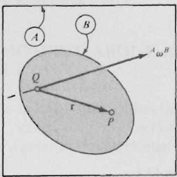
Figure 4.1.2

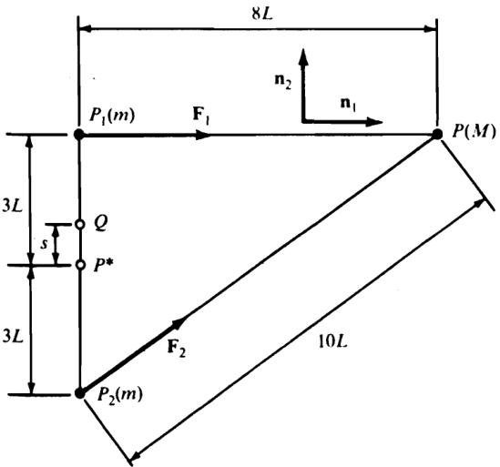
Figure 4.1.3

P_{1},\dots,P_{v} in A , is regarded as a bound vector whose line of action passes through an arbitrary point Q , then the angular momentum of S relative to any other point o is equal to the sum of the angular momentum of S relative to Q in A and the moment, about point o ,of the linear momentum of s in A

As a final example, consider the set of three particles P_{1},P_{2} , and P shown in Fig. 4.1.3, and let P_{1} and P_{2} each have a mass m while P has a mass M In accordance with Newton's law of gravitation, the gravitational forces. \mathbf{F}_{1} and \mathbf{F}_{2} . exerted, respectively, on \boldsymbol{P}_{1} and P_{2} by P have the lines of action shown in Fig. 4.1.3 and are given by

\mathbf{F}_{1}=\frac{G M m}{64L^{2}}\,\mathbf{n}_{1}\qquad\mathbf{F}_{2}=\frac{G M m}{100L^{2}}(0.8\mathbf{n}_{1}+0.6\mathbf{n}_{2})

where G is the universal gravitational constant, ^{\dagger} and \mathbf{n}_{1} and \scriptstyle\mathtt{\mathtt{n}}_{2} are unit vectors directed as shown. Under these circumstances, there exists a point Q on line P^{*}P_{1} ,where P^{*} is the mass center of \boldsymbol{P}_{1} and \boldsymbol{P}_{2} , such that \mathbf{M}^{Q}. the resultant of the moments of \mathbf{F}_{1} and \mathbf{F}_{2} about Q , is equal to zero. To locate Q, let s be the distance from P* to Q, as shown in Fig. 4.1.3, and let pi and p2 be the position vectors from Q to P_{1} and P_{2} , respectively. Then

{\bf p}_{1}=(3L-s){\bf n}_{2}\qquad{\bf p}_{2}=-(3L+s){\bf n}_{2}

and

{\bf M}^{Q}={\bf p}_{1}\times{\bf F}_{1}+{\bf p}_{2}\times{\bf F}_{2}\quad=\quad-\frac{G M m}{L^{2}}\Biggl[\frac{3L-s}{64}-\frac{(3L+s)(0.8)}{100}\Biggr]{\bf n}_{1}\times{\bf n}_{2}.

• G ≈ 6.6732 × 10-11 N m2 kg-2 (see E. A. Mechtly. "The International System of Units: Physical Constants and Conversion Factors." NASA SP-7012. revised, 1969).

Consequently, \mathbf{M}^{Q} vanishes when

s=0.968L

4.2 COUPLES, TORQUE

A couple is a set of bound vectors (see Sec. 4.1) whose resultant (see Sec.4.1) is equal to zero.A couple consisting of only two vectors is called a simple couple. Hence, the vectors forming a simple couple necessarily have equal magnitudes andoppositedirections.

Couples are not vectors,for a set of vectors is not a vector, any more than a set of points is a point; but there exists a unique vector, called the torque of the couple,that is intimately associated with a couple,namely,the moment of the couple about a point. It is unique because, as can be seen by reference to Eq. (4.1.3), a couplehas thesamemomentabout allpoints.

Example Four forces, \mathbf{F}_{1},\ldots,\mathbf{F}_{4} , have the lines of action shown in Fig. 4.2.1, and the magnitudes of \mathbf{F}_{1},\ldots,\mathbf{F}_{4} are proportional to the lengths of the lines A B ,BC, C D ,and D A ,respectively; that is,

\begin{array}{r l r l}&{\mathbf{F}_{1}=k a\mathbf{n}_{2}}&&{\mathbf{F}_{2}=k(-b\mathbf{n}_{1}+c\mathbf{n}_{3})}\\ &{\mathbf{F}_{3}=k(b\mathbf{n}_{1}-a\mathbf{n}_{2})}&&{\mathbf{F}_{4}=-k c\mathbf{n}_{3}}\end{array}

where k is a constant and {\bf n}_{1},\,{\bf n}_{2}\,,\,{\bf n}_{3} aremutually perpendicular unit vectors. The forces \mathbf{F}_{1},\ldots,\mathbf{F}_{4} form a couple since their resultant, \mathbf{F}_{1}+\mathbf{F}_{2}+\mathbf{F}_{3}+\, \mathbf{F}_{4} ,is equal to zero.The torque \mathrm{\bfT} ofthecouple,found,forexample,by adding themoments of \mathbf{F}_{1} \mathbf{F}_{4} aboutpoint C isgivenby(notethatthemoments of \mathbf{F}_{2} and \mathbf{F}_{3} about \scriptscriptstyle\cal{C} areequal tozero)

{\begin{array}{r l}&{{\mathbf{T}}=\left(-c\mathbf{n}_{3}+b\mathbf{n}_{1}\right)\times\mathbf{F}_{1}+\left(b\mathbf{n}_{1}-a\mathbf{n}_{2}\right)\times\mathbf{F}_{4}}\\ &{\qquad={\phantom{-}}k(2c a\mathbf{n}_{1}+b c\mathbf{n}_{2}+a b\mathbf{n}_{3})}\\ &{\qquad(1,2)}\end{array}}

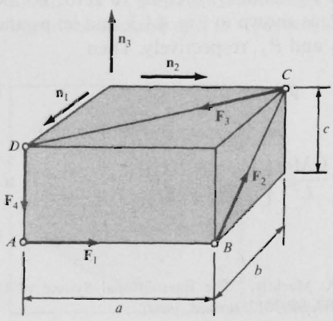
Figure 4.2.1

4.3 EQUIVALENCE, REPLACEMENT

Two sets of bound vectors are said to be equivalent when they have equal resultants and equal moments about one point; either set then is called a replacement of the Other.

Two couples having equal torques are equivalent, for they necessarily have equal resultants (zero; see Sec. 4.2) and their respective moments about every point are equal to each other because each such moment is equal to the torque of the corresponding couple.

When two sets of bound vectors, say, S and s^{\prime} , are equivalent, they have equal moments about every point. To see this, let s and s^{\prime} have equal resultants, and let Q be one point about which s and s^{\prime} have equal moments; then note that, in accordance with Eq. (4.1.3), the moments of s and s^{\prime} about any point \pmb{P} other than Q depend solely on the moments of s and S^{\prime} about Q , equal by hypothesis, and on the resultants of S and s^{\prime} , also equal by hypothesis.

If S is any set of bound vectors while S^{\prime} is a set of bound vectors consisting of a couple c of torque T together with a single bound vector \mathbf{v} whose line of action passes through a point P selected arbitrarily, then the following two requirements must be satisfied in order for s^{\prime} to be a replacement of s;\mathbf{T} is equal to the moment of S about P and vis equal to the resultant of S. For, when one of these requirements is violated, s and s^{\prime} either have unequal resultants or there exists no point about which s and s^{\prime} have equal moments. Conversely, satisfying both requirements guarantees the equivalence of s and S^{\prime} . These facts enable one to deal in simple analytical terms with sets of bound vectors, such as contact forces exerted by one body on another, in situations in which little is known about the individual vectors of such a set.

Example Figure 4.3.1 is a schematic representation of a device known as Hooke's joint, described as follows. Two shafts, s and s^{\prime} , are mounted in bearings, \boldsymbol{B} and \pmb{B}^{\prime} , which are fixed in a reference frame \pmb R . The axes of S and s^{\prime} are parallel to unit vectors n and {\bf{n}}^{\prime} , respectively, and intersect at a point \pmb{A} Each shaft terminates in a “ yoke,” and these yokes, Y and Y^{\prime} , are connected to each other by a rigid cross c , one of whose arms is supported by bearings at \pmb{D} and E in \boldsymbol{Y}, the other by bearings at D^{\prime} and E^{\prime} in Y^{\prime} . The two arms of c have equal lengths and form a right angle with each other. Furthermore, the arm supported by Y is perpendicular to n, while the one supported by Y^{\prime} is perpendicular to \ensuremath{\mathbf{n}}^{\prime} . Finally, circular disks G and G^{\prime} having radii r and \boldsymbol{r^{\prime}} are attached to s and s^{\prime} , respectively, and each of these is subjected to the action of a tangential force, one having a magnitude F and point of application \pmb{P} the other a magnitude of F^{\prime} and point of application P^{\prime}

In order for the system formed by G,G^{\prime},S,S^{\prime},Y,Y^{\prime} , and C to be in equilibrium, the ratio F/F^{\prime} must be related suitably to r,\;r^{\prime},\,\mathfrak{n},\,\mathfrak{n}^{\prime},\,\mathfrak{n} , and \pmb{v}^{\prime} ,where \pmb{\nu} and \pmb{v}^{\prime} are unit vectors parallel to the arms of {c} as shown in Fig. 4.3.1. To determine this relationship, one may consider the equilibrium of each of three rigid bodies, namely, the rigid body Z formed by G,S, and Y. the rigid body Z^{\prime} consisting of G', S', and Y', and the body C. The first of these is depicted in Fig. 4.3.2, where the vectors α, A, β, and B are associated with replacements of sets of contact forces exerted on Z by C and by the bearing at B. Specifically, the set of contact forces exerted on Z by C across the bearing surfaces at D and E is replaced with a couple of torque \pmb{\alpha} together with a force \mathbf{A} whose line of action passes through point A , and the set of contact forces exerted on Z by the bearing at \boldsymbol{B} is replaced with a couple of torque \upbeta togetherwithaforce \mathbf{B} whose line of action passes through the center of G. The vectors \alpha,\mathbf{A},\beta and \mathbf{B} are unknown,but,assuming that ail bearing surfaces are so smooth that the associated contact forces have lines of action normal to the surfaces, one can conclude that \pmb{\alpha} must be perpendicular to \mathbf{\Deltav} and \upbeta to \mathbf{u} sothat

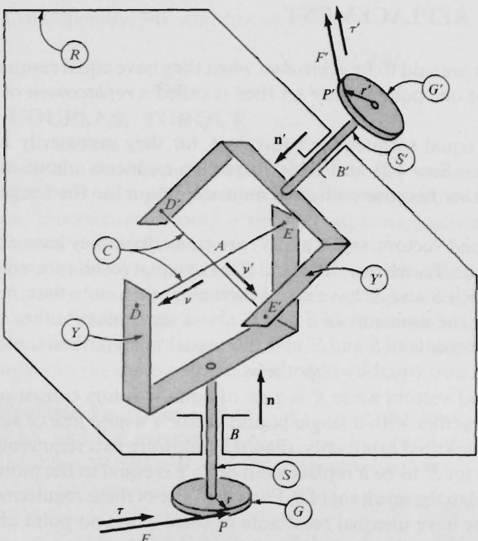
Figure 4.3.1

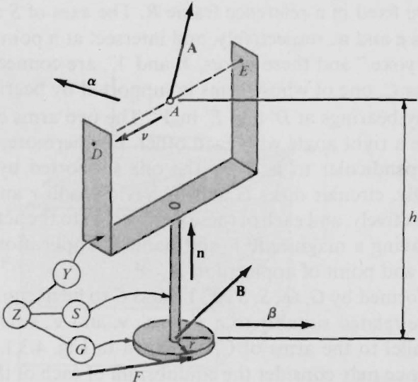
Figure 4.3.2

\mathbf{v}\cdot{\pmb{\alpha}}=0

and

{\mathfrak{n}}\cdot{\mathfrak{k}}=0

Now,when \angle is in equilibrium, the sum of the moments of all forces acting on \angle about the center of G is equal to zero.Hence, treating gravitational forces as negligible,one can write (see Fig.4.3.2 for h

r F\mathbf{n}+\alpha+\beta+h\mathbf{n}\times\mathbf{A}=0

and dot-multiplication of this equation with \mathbf{n} yields[when Eq. (2) is taken intoaccount]

\quad r F+\mathbf{n}\cdot{\mathsf{d}}=0

The body Z^{\prime} and vectors \pmb{\alpha}^{\prime},\mathbf{A}^{\prime},\pmb{\beta}^{\prime} , and \mathbf{B}^{\prime} respectively analogous to \propto A,β, and \mathbf{B} are shown in Fig.4.3.3.Reasoning as before,one finds that

\begin{array}{r}{\nu^{\prime}\cdot\alpha^{\prime}=0}\\ {\mathfrak{n}^{\prime}\cdot\mathfrak{B}^{\prime}=0}\end{array}

and

r^{\prime}F^{\prime}+\mathbf{n}^{\prime}\cdot\mathbf{\alpha}^{\prime}=0

Finally,in Fig.4.3.4, \zeta is shown together with vectors representing the sets ofcontactforcesexerted on C by Y and Y^{\prime} Thesevectorsarelabeled \rightharpoonup -\infty^{\prime} -\mathbf{A} and -\mathbf{A}^{\prime} in accordancewith the lawof action andreaction; that is,since to every force exerted on Y by C there corresponds aforce exerted

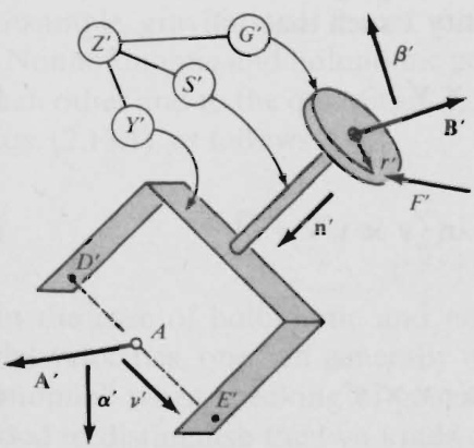
Figure 4.3.3

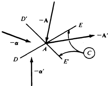
Figure 4.3.4

on C by \boldsymbol{Y}, these two forces having equal magnitudes, the same line of action, but opposite senses, it follows from the definition of a replacement of a set of bound vectors that, if the set of forces exerted on \boldsymbol{Y} by C is replaced with a couple of torque \pmb{\upalpha} together with a force A whose line of action passes through point A , while the set of forces exerted on c by \boldsymbol{Y} is replaced with a couple of torque \tilde{\pmb{\alpha}} together with a force \tilde{\mathbf{A}} whose line of action passes through point A then \tilde{\pmb{\alpha}}=-\pmb{\alpha} and \tilde{\mathbf{A}}=-\mathbf{A}. . Similar considerations apply to the interaction of ^{c} with Y^{\prime}

Because C_{} is presumed to be in equilibrium, the sum of the moments about point A of all forces acting on _{c} may be set equal to zero, so that, in view of Fig. 4.3.4, one can write

-a-a^{\prime}=0

Using this equation to eliminate \pmb{\alpha}^{\prime} from Eqs. (5) and (7), one arrives at

\mathbf{v}^{\prime}\cdot{\pmb{\alpha}}=0

and

r^{\prime}F^{\prime}-\boldsymbol{\mathsf{n}}^{\prime}\cdot\boldsymbol{\mathsf{a}}\,=\,0

Furthermore, Eqs. (1) and (9) show that \pmb{\upalpha} is perpendicular both to \pmb{\nu} and to \pmb{v}^{\prime} , which means that there exists a quantity \lambda such that

{\pmb{\alpha}}=\lambda{\pmb{v}}\times{\pmb{v}}^{\prime}

Consequently,

r F\underset{(4,11)}{=}-\lambda\mathbf{n}\cdot\mathbf{v}\,\times\,\mathbf{v}^{\prime}

while

r^{\prime}F^{\prime}\underset{(10,11)}{=}\lambda\mathbf{n}^{\prime}\cdot\mathbf{v}\,\times\,\mathbf{v}^{\prime}

Hence, the desired expression for F/F^{\prime} is

{\frac{F}{F^{\prime}}}\mathop{=}_{(12,13)}-{\frac{r^{\prime}\mathbf{n}\cdot\mathbf{v}\,\times\,\mathbf{v}^{\prime}}{r\mathbf{n}^{\prime}\cdot\mathbf{v}\,\times\,\mathbf{v}^{\prime}}}

What is most important here is to realize that it was possible to determine the relationship between F/F^{\prime} and r,\;r^{\prime},\;\mathfrak{n},\;\mathfrak{n}^{\prime},\;\mathfrak{v} , and \mathbf{v^{\prime}} despite the fact that relatively little is known about the contact forces exerted on s by the bearing B on Y by C , and so forth, and that the introduction of torques together with forces having well-defined lines of action greatly facilitated the solution process.

The method just used to arrive at Eq. (14) has one major faw, which is that it involves steps the motivation for which is not necessarily obvious, such assetting thesum of themoments of allforces actingon Z aboutthecenterof G equal to zero, dot-multiplying Eq. (3) with n, and so forth. In the example in Sec. 4.5 it is shown how Eq. (14) can be obtained in a more straightforward way.

4.4 GENERALIZED ACTIVE FORCES

Ⅱ \mathbf{\dot{\boldsymbol{u}}}_{1},\ldots,\mathbf{\boldsymbol{u}}_{n} are generalized speeds for a simple nonholonomic system s possessing p degrees o freedom in a reference frame A (see Sec.2.13), p quantities \boldsymbol{\tilde{F}}_{1},...,\boldsymbol{\tilde{F}}_{p} callednonholonomicgeneralizedactiveforcesfor s .n A and n quantities F_{1},\ldots,F_{n} called holonomic generalized active forces for s in A , are defined as

\widetilde{F}_{r}\triangleq\sum_{i\,=\,1}^{\nu}\widetilde{\mathbf{v}}_{r}^{\,\,P_{i}}\cdot{\mathbf{R}}_{i}\qquad(r=1,\ldots,p)

and

F_{r}\triangleq\sum_{i=1}^{v}\mathbf{v}_{r}^{\,P_{i}\,\cdot}\,{\bf R}_{i}\qquad(r=1,\ldots,n)

respectively, where \upnu is the number of particles comprising S, {\mathbf{}}P_{i} is a typical particle of s,\,\tilde{\mathbf{v}}_{r}^{\,\,P_{i}} and \mathbf{v}_{r}^{\,\,p_{i}} are, respectively, a nonholonomic partial velocity of \boldsymbol{P}_{i} in A and a holonomic partial velocity of P_{i} in A (see Sec. 2.14), and \mathbf{R}_{i} is the resultant (see Sec. 4.1) of ali contact forces for exampie, friction forces) and distance forces (for example, gravitational forces, magnetic forces, and so forth) acting on \boldsymbol{P}_{i}

Nonholonomic and holonomic generalized active forces for s in A are related to each other and to the quantities A_{r s}\left(s=1,\ldots,p;r=p+1,\ldots,n\right) introduced in Eqs. (2.13.1), as follows:

\tilde{F}_{r}=F_{r}+\sum_{s\,=\,p+1}^{n}F_{s}\,A_{s r}\qquad(r\,=\,1,\ldots,p)

As in the case of holonomic and nonholonomic partial angular velocities and partial velocities, one can generally omit the adjectives “holonomic” and “nonholonomic” when speaking of generalized forces, but the tilde notation should be used to distinguish the two kinds of generalized active forces from each other.

Derivation Referring to Eq. (2.14.17) to express \tilde{\mathbf{v}}_{r}^{\;\,P_{i}}\;(r=1,\dots,p) in termsof \mathbf{v}_{s}^{\,\,p_{i}} s=p+1,\ldots,n) ,onehas

\begin{array}{l}{{\displaystyle{\widetilde F}_{r}=\sum_{\scriptscriptstyle(1)\;i=1}^{\nu}\left({\bf v}_{r}{}^{P_{i}}+\sum_{\scriptscriptstyle s=p+1}^{n}{\bf v}_{s}{}^{P_{i}}A_{s r}\right)\cdot{\bf R}_{i}}\ ~}\\ {{\displaystyle=\sum_{i=1}^{\nu}{\bf v}_{r}{}^{P_{i}}\cdot{\bf R}_{i}+\sum_{\scriptscriptstyle s=p+1}^{n}\left(\sum_{\scriptscriptstyle i=1}^{\nu}{\bf v}_{s}{}^{P_{i}}\cdot{\bf R}_{i}\right)A_{s r}}\qquad(r=1,\ldots,p)}\end{array}

and use of Eqs. (2) then leads immediately to Eqs. (3).

Example In Fig. 4.4.1, \boldsymbol{P}_{1} and P_{2} designate particles of masses m_{1} and m_{2} that can slidefreelyin a smooth tube T and are attached to light linear springs \sigma_{1} and o_{2} having spring constants k_{1} and k_{2} and “natural" lengths L_{1} and L_{2} T ismadetorotate aboutafixedhorizontal axispassingthroughoneend of T in such a way that the anglebetween thevertical and the axis of T is a prescribed function \theta(t) of the time t Generalized active forces \boldsymbol{F}_{1} and \boldsymbol{F}_{2} associatedwithgeneralizedspeeds \boldsymbol{u}_{1} and u_{2} defined as

u_{r}\triangleq\dot{q}_{r}\qquad(r=1,2)

are to be determined for the system S formed by the two particles \boldsymbol{P}_{1} and P_{2} ， with q_{1} and q_{2} (see Fig. 4.4.1) designating the displacements of \boldsymbol{P}_{1} and P_{2} from the positions occupied by \boldsymbol{P}_{1} and P_{2} in T when \sigma_{1} and \sigma_{2} are undeformed.

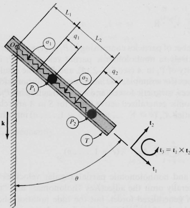
The velocities \mathbf{v}^{P_{1}} and \mathbf{v}^{P_{2}} of P_{1} and P_{2} can be expressed as (see Fig. 4.4.1 for the unit vectors {\bf f}_{1} and {\bf f}_{2}

\begin{array}{r l}&{\mathbf{v}^{P_{1}}\quad=\quad u_{1}\mathbf{t}_{1}+(L_{1}+q_{1})\dot{\theta}\mathbf{t}_{2}}\\ &{\quad\quad\quad^{(2.8.1)}\quad\quad\quad\quad\quad\quad\quad\quad\cdot}\\ &{\quad\quad\mathbf{v}^{P_{2}}\quad=\quad u_{2}\mathbf{t}_{1}+(L_{1}+L_{2}+q_{2})\dot{\theta}\mathbf{t}_{2}}\\ &{\quad\quad\quad(2.8.1)\quad\quad\quad\quad\quad}\end{array}

s is a holonomic system, and the partial velocities of P_{1} and P_{2} are

\begin{array}{r l}{\mathbf{v}_{1}{}^{P_{1}}=\mathbf{t}_{1}\quad}&{{}\mathbf{v}_{2}{}^{P_{1}}=0}\\ {\mathbf{\eta}_{(6)}^{(6)}\quad}&{{}\mathbf{\Gamma}_{(6)}^{(6)}}\\ {\mathbf{v}_{1}{}^{P_{2}}=0\quad}&{{}\mathbf{v}_{2}{}^{P_{2}}=\mathbf{t}_{1}}\\ {\mathbf{\eta}_{(7)}^{(7)}\quad}&{{}\mathbf{\Gamma}_{(7)}^{(7)}}\end{array}

Contact forces are applied to \boldsymbol{P}_{1} by \sigma_{1},\sigma_{2} , and T , and a gravitational force is exerted on P_{1} by the Earth. The forces applied to P_{1} by \sigma_{1} and \sigma_{2} can be written -k_{1}q_{1}\mathbf{t}_{1} and k_{2}(q_{2}-q_{1})\mathbf{t}_{1} , respectively, and the force exerted on \boldsymbol{P}_{1} by T can be expressed as T_{12}\mathbf{t}_{2}+\ T_{13}\mathbf{t}_{3} ,where T_{12} and T_{13} are unknown scalars. No component parallel to {\bf f}_{1} is included because T is presumed to be smooth. Finally, the gravitational force exerted on P_{1} by the Earth is m_{1}g\mathbf{k} where \boldsymbol{g} is the local gravitational acceleration and \mathbf{k} is a unit vector directed vertically downward. Hence if the gravitational force exerted on \boldsymbol{P}_{1} by P_{2} is ignored, \mathbb{R}_{1} , the resultant of all contact and distance forces acting on P_{1} , is given by

\mathbf{R}_{1}\,=\,-k_{1}q_{1}\mathbf{t}_{1}\,+\,k_{2}(q_{2}\,-\,q_{1})\mathbf{t}_{1}\,+\,T_{12}\,\mathbf{t}_{2}\,+\,T_{13}\,\mathbf{t}_{3}\,+\,m_{1}g\mathbf{k}

and (F_{\uparrow})_{P_{1}} , the contribution to the generalized active force F_{1} of all contact and distance forces acting on P_{1} ,is

(F_{1})_{P_{1}}=\mathbf{v}_{1\atop(2)}^{\mathbf{\alpha}_{1}\mathbf{\alpha}_{1}}\mathbf{\cdot}\mathbf{R}_{1}\underset{(8,10)}{=}-k_{1}q_{1}+k_{2}(q_{2}-q_{1})+m_{1}g\cos{\theta}

Similarly, the resultant \mathbf{R}_{2} of all contact and distance forces acting on P_{2} is

{\bf R}_{2}=\,-k_{2}({q_{2}}\mathrm{~-~}{q_{1}}){\bf t}_{1}\,+\,T_{22}\,{\bf t}_{2}\,+\,T_{23}\,{\bf t}_{3}\,+\,m_{2}\,g{\bf k}

so that (F_{1})_{P_{2}} , the contribution to the generalized active force F_{1} of all contact and distance forces acting on P_{2} ,is

(F_{1})_{P_{2}}={\mathbf{v}_{1}}^{P_{2}}\cdot{\mathbf{R}_{2}}\mathbf{\Phi}=\mathbf{\Phi}0

and, proceeding in the same way, one finds that (F_{2})_{P_{1}} and (F_{2})_{P_{2}} , the contributions to the generalized active force F_{2} of all contact and distance forces acting on \boldsymbol{P}_{1} and P_{2} , respectively, are

(F_{2})_{P_{1}}={\bf v}_{2}{}^{P_{1}}\cdot{\bf R}_{1}\;\;=\;\;0

and

(F_{2})_{P_{2}}={\bf v_{\mathrm{2}}}^{P_{2}}\cdot{\bf R_{\mathrm{2}}}\;\;=\;\;-k_{2}(q_{2}-q_{1})+m_{2}g\,\cos\theta

The desired generalized active forces are thus

F_{1}=(F_{1})_{P_{1}}+(F_{1})_{P_{2}}\underset{(11,13)}{=}-k_{1}q_{1}+k_{2}(q_{2}-q_{1})+m_{1}g\cos{\theta}

and

F_{2}\,=\,(F_{2})_{P_{1}}+\,(F_{2})_{P_{2}}\underset{(14,15)}{=}\,-k_{2}(q_{2}\,-\,q_{1})\,+\,m_{2}\,g\,\cos\theta

It is worth noting that the (unknown) contact forces exerted on P_{1} and P_{2} by T contribute nothing to the generalized active forces F_{1} and F_{2}

4.5 NONCONTRIBUTING FORCES

Some forces that contribute to \mathbf{R}_{i} as defined in Sec. 4.4 make no contributions to the generalized active forces \widetilde{F} (r=1,\ldots,p) or, if s is a holonomic system, to the generalized active forces F_{\prime} (r=1,\ldots,n) . Indeed, this is the principal motivation for introducing generalized active forces. For example, the total contribution to \tilde{F}_{r} of all contact forces exerted on particles of S across smooth surfaces of rigid bodies vanishes; if B is a rigid body belonging to s , the total contribution to \widetilde{F}_{r} of all contact and distance forces exerted by all particles of B On each other is equal to zero; when B rolls without slipping on a rigid body B^{\prime} , the total contribution to \widetilde{F}_{r} of all contact forces exerted on B by B^{\prime} is equal to zero if B^{\prime} is not a part of S and the total contribution to \widetilde{F}_{r} of all contact forces exerted by B and B^{\prime} on each other is equal to zero if B^{\prime} is a part of s

Derivations Let \mathbf{C} be a contact force exerted on a particle P of s by a rigid body B across asmoothsurface of B Then, if \bar{\mathbf{n}} is a unit vector normal to the surface of B at P

\mathbf{C}=C\mathbf{n}

where C is some scalar. Now consider A_{\mathbf{v}}P , the velocity of P in A , which can be expressed as

\begin{array}{r}{\mathbf{\Pi}^{A}\mathbf{v}^{P}\quad=\quad\mathbf{\Pi}^{A}\mathbf{v}^{\ddot{B}}\,+\,^{B}\mathbf{v}^{P}\,}\\ {(2.8.1)\qquad\qquad\qquad\qquad\quad}\end{array}

where A_{\mathbf{V}}\tilde{B} is the velocity in A of the point \bar{B} of B that is in contact with P and \pmb{{\cal B}}_{\mathbf{v}}P is the velocity of P in B If P is neither to lose contact with B nor to penetrate \boldsymbol{B} then \pmb{B}_{\mathbf{v}}P must be perpendicular to n, and this means that

B_{\widetilde{\mathbf{V}}_{r}}{}^{P}\cdot\mathfrak{n}=0\qquad(r=1,\dotsc,p)

because otherwise there can exist values of such that \mathbf{\Delta}^{B}\mathbf{v}^{P} is not perpen$u_{1},,\cdot,\cdot$ u_{p} dicular to \boldsymbol{\mathfrak{u}} Suppose that B is part of {\cal{S}} Then [see Eq. (2.14.4)]

^{A}\tilde{\mathbb{V}}_{r}^{\textit{P}}={}^{A}\tilde{\mathbb{V}}_{r}^{\textit{B}}+{}^{B}\tilde{\mathbb{V}}_{r}^{\textit{P}}~~~~~~(r=1,\dots,p)

Consequently,

(^{A}\tilde{\mathbf{v}}_{r}^{~P}-{^{A}\tilde{\mathbf{v}}_{r}^{~B}})\cdot\mathbf{n}={^{B}\tilde{\mathbf{v}}_{r}^{~P}}\cdot\mathbf{n}=0~~~~~~(r=1,\ldots,p)

and the contribution to {\tilde{F}}_{r} of the forces exerted on each other by P and B is[see Eq. (4.4.1)]

A_{\tilde{\mathbf{V}}_{r}}\mathbf{\mathcal{P}}\cdot(C\mathbf{n})+{}^{A_{\tilde{\mathbf{V}}_{r}}\tilde{B}}\cdot(-C\mathbf{n})=C(^{A_{\tilde{\mathbf{V}}_{r}}\tilde{P}}-{}^{A_{\tilde{\mathbf{V}}_{r}}\tilde{B}})\cdot\mathbf{n}=0\qquad(r=1,\ldots,p)

Alternatively, if B is not part of {\cal{S}} ,then u_{1},\dotsc,u_{p} always can be chosen in such a way that A_{\mathbb{V}}B is independent of u_{1},\dotsc,u_{p} ,in which event

^{A}\tilde{\mathbf{v}}_{r}^{~P}={^{B}\tilde{\mathbf{v}}_{r}^{~P}}~~~~~~(r=1,...,p)

and the contribution to \scriptstyle{\vec{F}}_{r} of the contact force exerted by B on P is [seeEq.(4.4.1)]

^{A}\tilde{\mathbf{y}}_{r}^{~P}\cdot(C\mathbf{n})=C^{B}\tilde{\mathbf{v}}_{r}^{~P}\cdot\mathbf{n}=0~~~~~~(r=1,\ldots,p)

In both cases it thus follows that the total contribution to \bar{\boldsymbol{F}}_{r} of all contactforces exertedonparticlesof {\cal{S}} across smooth surfaces of rigid bodies vanishes.

In Fig. 4.5.1, P_{i} and P_{j} designate any two particles of a rigid body B belonging to {\cal{S}} \mathbb{R}_{i j} is the resultant of all contact and distance forces exerted on P_{i} by P_{j} and \mathbb{R}_{j i} is the resultant of all contact and distance forces exerted on P_{j} by P_{i} We shall show that the total contribution of {\mathbf{R}}_{i j} and \mathbf{R}_{j i} to \tilde{F}_{r} r=1,\hdots,p) is equal to zero,from which it follows that the total contribution to \scriptstyle{\vec{F}}_{r} ofall contact and distance forces exerted by all particles of B on each other is equal to zero.

The partiai velocities ^{A}\widetilde{\mathbf{V}}_{r}^{~P_{i}} and ^{A}\widetilde{\mathbf{y}}_{r}^{\,\,\,P_{j}} of P_{i} and P_{j} in A are related to thepartial angular velocity ^A\tilde{\mathbf{w}}_{r}^{B} of B in A by [see Eqs. (2.7.1), (2.14.3), and (2.14.4)]

A_{\widetilde{\mathbf{V}}_{r}}^{\widetilde{\mathbf{\Gamma}}_{P_{j}}}=\mathbf{\widetilde{\omega}}_{\widetilde{\mathbf{V}}_{r}}^{A_{\widetilde{\mathbf{\Gamma}}}}P_{i}^{\mathbf{\Gamma}_{i}}+\mathbf{\widetilde{\omega}}_{\widetilde{\mathbf{0}}_{r}}^{A_{\widetilde{\mathbf{\Gamma}}}}\times\mathbf{\widetilde{p}}_{i j}\qquad(r=1,\ldots,p)

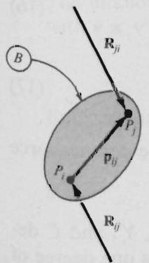
Figure 4.5.1

where \mathbf{p}_{i j} is the positionvector from {\mathbf{}}P_{i} to P_{j} ; and the forces \mathbb{R}_{i j} and \mathbb{R}_{j i} are related to each other by the law of action and reaction, which asserts that \mathbb{R}_{i j} and \mathbb{R}_{j i} have equal magnitudes, opposite directions, and coincident lines of action. Hence,

{\mathbb R}_{j i}=-{\mathbb R}_{i j}

and, since the line of action of \mathbb{R}_{i j} passes through {\mathbf{}}P_{i} , it is parallel to \pmb{\mathrm{p}}_{i j} ,which meansthat

\mathsf{p}_{i j}\times\,\mathsf{R}_{i j}=0

Consequently, the total contribution of \mathbf{R}_{i j} and \mathbb{R}_{j i} to \widetilde{F}_{r}\ (r=1,\ldots,p) is [see Eq. (4.4.1)]

\begin{array}{r l}{{^{A}\tilde{\mathbf{v}}_{r}}^{P_{i}}\cdot\mathbf{R}_{i j}+{^{A}\tilde{\mathbf{v}}_{r}}^{P_{j}}\cdot\mathbf{R}_{j i}=}&{({^{A}\tilde{\mathbf{v}}_{r}}^{P_{i}}-{^{A}\tilde{\mathbf{v}}_{r}}^{P_{j}})\cdot\mathbf{R}_{i j}}\\ {{^(10)}}&{}\\ {=-{^{A}\tilde{\mathbf{0}}_{r}}^{B}\times\ \mathbf{p}_{i j}\cdot\mathbf{R}_{i j}=\mathbf{0}\quad\quad(r=1,\ldots,p)}\end{array}

Finally, to deal with contact forces that come into play when \boldsymbol{B} rolls on a rigid body \mathbf{\deltaB^{\prime}} , we let P be a point of \boldsymbol{B} , and P^{\prime} a point of B^{\prime} , choosing these such that P is in rolling contact with P^{\prime} ,whichmeansthat

A_{\mathbf{v}}P_{\mathbf{\Phi}}=A_{\mathbf{v}}P^{\prime}

where A is any reference frame. Now there are two possibilities. Either B^{\prime} belongs to s_{\mathrm{:}} inwhich case

^{A}\tilde{\Psi}_{r}^{~~P}~=~^{A}\tilde{\Psi}_{r}^{~P^{\prime}}~~~~~~~(r=1,\,.\,.\,.\,,p)

and the contribution to {\widetilde{\boldsymbol{F}}}_{r} of \mathbf{R} and \mathbf{R}^{\prime} , the resultants of the contact forces exerted by B^{\prime} on \boldsymbol{B} and by \boldsymbol{B} on B^{\prime} , respectively, is given by

{}^{A}\tilde{\mathbf{v}}_{r}{}^{P}\cdot\mathbf{R}\,+\,{}^{A}\tilde{\mathbf{v}}_{r}{}^{P^{\prime}}\cdot\mathbf{R}^{\prime}\,=\,{}^{A}\tilde{\mathbf{v}}_{r}{}^{P}\cdot(\mathbf{R}\,+\,\mathbf{R}^{\prime})

which vanishes because, in accordance with the law of action and reaction, \textstyle\mathbf{R}+ \mathbf{R}^{\prime}=0 Alternatively, B^{\prime} does not belong to s , in which case generalized speeds always can be chosen such that A_{\mathbf{v}}P^{\prime} is independent of all of them, so that

^{A}\tilde{\upnu}_{r}{}^{P^{\prime}}=0\qquad(r=1,\ldots,p)

and, consequently,

A_{\widetilde{\mathbf{V}}_{r}}^{A}P\!\!\!\!\!\!\!_{(13,16)}\!\!\!\!\!\!\!0\!\!\!\!\!\!\!\!\!\!\!\!\!\!\!\!\!\!\!\!\!\!\!\!\!\!\!\!\!\!\!\!\!\!\!\!\!\!\!\!\!\!\!\!\!\!\!\!\!\!\!\!\!\!\!\!\!\!\!\!\!\!\!\!\!\!\!\!\!\!\!\!\!\!\!\!\!\!\!\!\!\!\!\!\!\!\!\!\!\!\!\!\!\!\!\!\!\!\!\!\!\!\!\!\!\!\!\!\!\!\!\!\!\!\!\!\!\!\!\!\!\!\!\!\!\!\!\!\!\!\!\!\!\!\!\!\!\!\!\!\!\!\!\!\!\!\!\!\!\!\!\!\!\!\!\!\!\!\!\!\!\!\!\!\!\!\!\!\!\!\!\!\!\!\!\!\!\!\!\!\!\!\!\!\!\!\!\!\!\!\!\!\!\!\!\!\!\!\!\!\!\!\!\!\!\!\!\!\!\!\!\!\!\!\!\!\!\!\!\!\!\!\!\!\!\!\!\!\!\!\!\!\!\!\!\!\!\!\!\!\!\!\!\!\!\!\!\!\!\!\!\!\!\!\!\!\!\!\!\!\!\!\!\!\!\!\!\!\!\!\!\!\!\!\!\!\!\!\!\!\!\!\!\!\!\!\!\!\!\!\!\!\!\!\!\!\!\!\!\!\!\!\!\!\!\!\!\!\!\!\!\!\!\!\!\!\!\!\!\!\!\!\!\!\!\!\!\!\!\!\!\!\!\!\!\!\!\!\!\!\!\!\!\!\!\!\!\!\!\!\!\!\!\!\!\!\!\!\!\!\!\!\!\!\!\!\!\!\!\!\!\!\!\!\!\!\!\!\!\!\!\!\!\!\!\!\!\!\!\!\!\!\!\!\!\!\!\!\!\!\!\!\!\!\!\!\!\!\!\!\!\!\!\!\!\!\!\!\!\!\!\!\!\!\!\!\!\!\!\!\!\!\!\!\!\!\!\!\!\!\!\!\!\!\!\!\!\!\!\!\!\!\!\!\!\!\!\!\!\!\!\!\!\!\!\!\!\!\!\!\!\!\!\!\!\!\!\

from which it follows that A_{\widetilde{\mathbf{v}}_{r}}\mathbf{\cdot}\mathbf{R}. the contribution to {\widetilde{\boldsymbol{F}}}, of the contact force exerted on B by B^{\prime} at P , is equal to zero.

Example The system \pmb{H} formed by the bodies G,\,G^{\prime},\,S,\,S^{\prime},\,Y,\,Y^{\prime} and C described in the example in Sec. 4.3 is holonomic and possesses one degree of

freedom in the reference frame \pmb R shown in Fig. 4.3.1. Defining a single generalized speed \pmb{u}_{1} as

u_{1}\triangleq^{R}\!\mathbf{\omega}\!\mathbf{\omega}^{G}\cdot\mathbf{n}

and letting R_{\mathbf{v}_{1}}{}^{P} and \boldsymbol{R}_{\mathbf{v}_{1}}\boldsymbol{P^{\prime}} denote the associated partial velocities of P and P^{\prime} respectively,in R , one can express the contribution of the forces of magnitudes F and F^{\prime} (see Fig. 4.3.1) to the generalized active force F_{1} for \pmb{H} in R as

F_{1}\,=\,^{R}\mathbf{v_{1}}^{P}\cdot(F\bar{\mathfrak{v}})\,+\,^{R}\mathbf{v_{1}}^{P^{\prime}}\cdot(F^{\prime}\bar{\mathfrak{v}}^{\prime})

where \mathfrak{c} and \pmb{\tau}^{\prime} are unit vectors parallel to the tangents to G and G^{\prime} at \pmb{P} and P^{\prime} respectively, as indicated in Fig. 4.3.1. Moreover, if it is assumed, as before, that all bearing surfaces are smooth, and if gravitational forces are once again left out of account, then F_{1} as given by Eq. (19) is, in fact, the total generalized activeforcefor H in \pmb R

In the example in Sec. 4.3, considerations of the equilibrium of each of three rigid bodies led to Eq. (4.3.14). The same result can be obtained simply by setting the generalized active force F_{1} equal to zero, which leads, first, to

\frac{F}{F^{\prime}}=\mathrm{~-~}\frac{\kappa_{{\mathbf{v}_{1}}}{\bf{\sigma}}^{P^{\prime}}\cdot{\bf{\sigma}}\cdot{\bf{\sigma}}^{\prime}}{R_{{\mathbf{v}_{1}}}{\bf{\sigma}}^{P}\cdot{\bf{\sigma}}\tau}

Now, with self-explanatory notation,

\mathbf{\nabla}^{R}\mathbf{\omega}^{S^{\prime}}\mathbf{\omega}=\mathbf{\omega}^{R}\mathbf{\omega}\mathbf{\omega}^{S}+\mathbf{\omega}^{S}\mathbf{\omega}^{C}+\mathbf{\omega}^{C}\mathbf{\omega}^{S^{\prime}}

and the simple angular velocities (see Sec. 2.2) appearing in this equation can beexpressed as

\begin{array}{r l}{\mathbf{\boldsymbol{^R_{\acute{\Theta}}}}^{S^{\prime}}=\mathbf{\boldsymbol{^R_{\acute{\omega}}}}^{S^{\prime}}\mathbf{\boldsymbol{n^{\prime}}}\qquad\qquad}&{{}\mathbf{\boldsymbol{^R_{\acute{\Theta}}}}^{S}\ =\ u_{1}\mathbf{\boldsymbol{n}}}\\ {\mathbf{\boldsymbol{^18}}\mathbf{\boldsymbol{^C}}=s_{\omega}c_{\mathbf{\boldsymbol{v}}}\qquad\qquad}&{{}c_{\mathbf{\boldsymbol{\Theta}}}s^{\prime}=c_{\boldsymbol{\omega}}s^{\prime}\mathbf{\boldsymbol{v}}}\end{array}

Hence,

^{R}\!{\omega}^{S^{\prime}}\mathbf{n}^{\prime}\;=\;u_{1}\mathbf{n}\,+\,^{s}\!{\omega}^{C}\!\mathbf{v}\,+\,^{c}\!{\omega}^{s^{\prime}}\mathbf{v}^{\prime}

The unknowns s_{\omega}c and c_{\omega}s^{\prime} can be eliminated by dot-multiplying Eq. (24) with \textbf{v}\times\textbf{v} , which gives

\scriptstyle{\boldsymbol{\kappa}}_{\omega}s^{\prime}\mathbf{n}^{\prime}\\cdot\,\mathbf{v}\ \times\ \mathbf{v}^{\prime}\ =\ u_{1}\mathbf{n}\cdot\mathbf{v}\ \times\ \mathbf{v}^{\prime}

Furthermore, the velocities of P and P^{\prime} in R are

^R{\mathbf{v}}^{P}=r u_{1}\boldsymbol{\tau}

and

^R_{\Psi}P^{\prime}=r^{\prime R}\omega^{S^{\prime}}\bar{\sftau}^{\prime}=\;r^{\prime}u_{1}\;\frac{{\sf n}\cdot{\sf v}\times{\bf\delta v}^{\prime}}{{\sf n}^{\prime}\cdot{\bf v}\times{\bf\delta v}^{\prime}}\bar{\sf\tau}^{\prime}

so that the partial velocities {{\boldsymbol{R}}_{\mathbf{v}_{1}}}{{\boldsymbol{P}}} and {{\mathcal{R}}_{\mathbf{V}_{1}}}^{p\prime} are given by

\begin{array}{r l r}{\displaystyle^{R}\mathbf{v}_{1}^{\mathrm{~\tiny~P~}}=\mathbf{\delta}r\bar{\mathbf{\tau}}}&{{}}&{\displaystyle^{R}\mathbf{v}_{1}^{\mathrm{~\tiny~P~}}=\mathbf{\delta}r^{\prime}\,\frac{\bar{\mathbf{n}}^{\mathrm{~\tiny~P~}}\times\mathbf{\delta}\mathbf{v}^{\prime}}{\bar{\mathbf{n}}^{\prime}\cdot\mathbf{v}\,\times\mathbf{\deltav}^{\prime}}\,\bar{\mathbf{\tau}}^{\prime}}\end{array}

Substitution from Eqs. (28) into Eq. (20) leads directly to Eq. (4.3.14)

4.6 FORCES ACTING ON A RIGID BODY

If \boldsymbol{B} is a rigid body belonging to a nonholonomic system S possessing p degrees of freedom in a reference frame A (see Sec. 2.13), and a set of contact and/or distance forces acting on B is equivalent (see Sec. 4.3) to a couple of torque \mathbf{T} (see Sec. 4.2) together with a force \mathbf{R} whose line of action passes through a point Q of B then (\tilde{\widetilde{F}}_{r})_{B} , the contribution of this set of forces to the generalized active force {\tilde{F}}, (see Sec. 4.4) for s in A is given by

(\widetilde{F}_{r})_{B}={}^{A}\tilde{\upomega}_{r}{}^{B}\cdot\mathrm{T}\,+\,{}^{A}\tilde{\upnu}_{r}{}^{Q}\cdot{\bf R}\qquad(r=1,\ldots,p)

where ^{A}\widetilde{\mathbf{G}}_{r}{^{B}} and {^{A}{\mathfrak{v}}_{r}}^{Q} are, respectively, the rth partial angular velocity of B in A and the rth partial velocity of Q in A

Derivation Let \mathbf{K}_{1}\,,\dots\,,\mathbf{K}_{\beta} be the contact and/or distance forces acting on particles P_{1},\ldots,P_{\beta} of \mathbfit{B} and let \mathfrak{p}_{1}\,,\,.\,.\,.\,,\,\mathfrak{p}_{\beta} be the position vectors from Q to P_{1},\ldots,P_{\beta} respectively. Then, by definition of equivalence, the resultant of \mathbf{K}_{1},\ldots,\mathbf{K}_{\beta} is equalto \mathbf{R} ,that is,

\sum_{i\mathop{=}1}^{\beta}\mathbf{K}_{i}\mathop{=}_{(4\cdot1\cdot2)}\mathbf{R}

and the sum of the moments of \mathbf{K}_{1},\ldots,\mathbf{K}_{\beta} about Q is equal to \mathbf{T} , so that

\sum_{i\,=\,1}^{\beta}\,\mathbf{p}_{i}\times\,\mathbf{K}_{i}=\,\mathbf{T}

Also by definition, the contribution of \mathbf{K}_{1},\ldots,\mathbf{K}_{\beta} to \widetilde{F}_{r} is

(\widetilde F_{r})_{B}\underset{(4,4,1)}{=}\sum_{i=1}^{\beta}\,A_{\widetilde{\mathbf{V}}_{r}}P_{i}\cdot\mathbf{K}_{i}\qquad(r=1,\ldots,p)

where, with the aid of Eqs. (2.7.1), (2.14.4), and (2.14.3), one can express A_{\widetilde{\mathbf{v}}_{r}}\mathbf{\widetilde{\mathbf{\Pi}}}^{P_{i}} as

A_{\widetilde{\mathbf{V}}_{r}}^{\widetilde{\mathbf{\Gamma}}_{r}}=\mathbf{\widetilde{\omega}}_{\widetilde{\mathbf{V}}_{r}}^{A}\mathbf{\mathcal{Q}}+\mathbf{\widetilde{\omega}}_{\widetilde{\mathbf{0}}_{r}}^{A}\mathbf{\mathcal{S}}\times\mathbf{p}_{i}\qquad(r=1,\ldots,p;i=1,\ldots,\beta)

Hence,

\begin{array}{r l r}&{}&{\langle(\widetilde F_{r})_{B}=\displaystyle\sum_{(4)\;i=1}^{\beta}({\}^{A}\widetilde{\mathbf v}_{r}{}^{Q}+{\}^{A}\widetilde{\mathbf o}_{r}{}^{B}\times{}\,\mathbf p_{i})\cdot\mathbf K_{i}={\}\widetilde{\mathbf v}_{r}{}^{Q}\cdot\displaystyle\sum_{i=1}^{\beta}\mathbf K_{i}+{\}\widetilde{\mathbf o}_{r}{}^{B}\cdot\displaystyle\sum_{i=1}^{\beta}\mathbf p_{i}\times{}\,\mathbf K_{i}}\\ &{}&{={\}^{A}\widetilde{\mathbf v}_{r}{}^{Q}\cdot\mathbf R{}_{*}+{\}^{A}\widetilde{\mathbf o}_{r}{}^{B}\cdot{}\mathbf T_{*}\qquad(r=1,\ldots,p)}\end{array}

in agreement with Eq. (1).

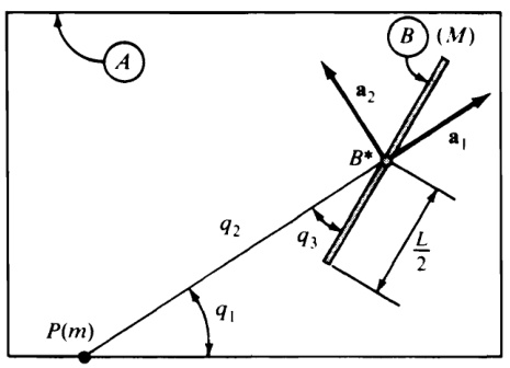
Figure 4.6.1

Example Figure 4.6.1 shows a uniform rod B of mass M and length L,\;B is free to move in a plane A , and P is a particle of mass m , fixed in A ：

It can be shownt that the set of gravitational forces exerted by P on B is approximately equivalent to a couple of torque \mathbf{T} togetherwithaforce \mathbf{R} whose line of action passes through the mass center B^{*} of B with \mathbf{T} and \mathbf{R} given by

\mathbf{T}=\mathbf{-}\ {\frac{G M m L^{2}}{8q_{2}{}^{3}}}\sin2q_{3}\mathbf{a}_{1}\ \times\ \mathbf{a}_{2}

and

{\bf R}=\mathrm{}-\frac{G M m}{{q_{2}}^{2}}\biggl\{{\bf a}_{1}\left[1+\frac{L^{2}}{8{q_{2}}^{2}}{(2-3\sin^{2}{q_{3}})}\right]-{\bf a}_{2}\frac{L^{2}}{8{q_{2}}^{2}}\sin{2q_{3}}\biggr\}

where G is the universal gravitational constant, \mathbf{a}_{1} and {\mathbf a}_{2} are unit vectors directed as shown in Fig. 4.6.1, and q_{1},\,q_{2},\,q_{3} are generalized coordinates characterizing the configuration of B in A (see Fig. 4.6.1). If generalized speeds u_{1},u_{2},u_{3} are introduced as

u_{r}\triangleq\dot{q}_{r}\qquad(r=1,2,3)

then \mathbf{\omega} , the angular velocity of B in A , and \mathbf{v} , the velocity of B^{*} in A , are given by

\mathbf{\omega}\mathbf{\omega}=(u_{1}+u_{3})\,\mathbf{a}_{1}\,\times\,\mathbf{a}_{2}\qquad\mathbf{v}=u_{2}\,\mathbf{a}_{1}\,+\,u_{1}q_{2}\,\mathbf{a}_{2}

so that the partial angular velocities of B in A and the partial velocities of B^{*} in A are

\begin{array}{c c c}{{\mathbf{\omega}_{0_{1}}=\mathbf{a}_{1}\,\times\,\mathbf{a}_{2}}}&{{}}&{{\mathbf{\omega}_{0_{2}}=0}}&{{\mathbf{\omega}_{0_{3}}=\mathbf{a}_{1}\,\times\,\mathbf{a}_{2}}}\\ {{\mathbf{\omega}_{1}=q_{2}\,\mathbf{a}_{2}}}&{{}}&{{\mathbf{\omega}_{\mathbf{\nu}_{2}}=\mathbf{a}_{1}}}&{{\mathbf{\omega}_{\mathbf{\nu}_{3}}=0}}\end{array}

• T. R. Kane, P. W. Likins, and D. A. Levinson, Spacecraft Dynamics (McGraw-Hill, New York. 1983), Secs. 2.3, 2.6.

The contributions of the gravitational forces exerted by P on \boldsymbol{B} to the generalized active forces for B in A are

\begin{array}{l c l}{{(F_{1})_{B}}}&{{=}}&{{{\bf4}_{1}\times{\bf~a}_{2}\cdot{\bf T}+q_{2}{\bf a}_{2}\cdot{\bf R}}}\\ {{}}&{{(1)}}&{{\quad\quad\quad(11)}}\\ {{}}&{{=}}&{{-\,\displaystyle\frac{G M m L^{2}}{8q_{2}^{3}}\sin2q_{3}+\displaystyle\frac{G M m L^{2}}{8q_{2}^{3}}\sin2q_{3}=0}}\\ {{}}&{{\quad\quad\quad(\frac{\sin2}{\sin})}}\\ {{(F_{2})_{B}}}&{{=}}&{{\displaystyle\frac{G M m}{q_{2}^{2}}\Biggl[1+\frac{L^{2}}{8q_{2}^{2}}(2-3\sin^{2}q_{3})\Biggr]}}\\ {{}}&{{\quad\quad(F_{3})_{B}=}}&{{-\,\displaystyle\frac{G M m L^{2}}{8q_{2}^{3}}\sin2q_{3}}}\end{array}

4.7 CONTRIBUTING INTERACTION FORCES

In Sec. 4.5 it was shown that certain interaction forces, that is, forces exerted by one part of a system on another, make no contributions to generalized active forces. In some situations, forces of interaction do contribute to generalized active forces. For example, whenever two particles of a system are not rigidly connected to each other, the gravitational forces exerted by the particles on each other can make such contributions. Bodies connected to each other by certain energy storage or energy dissipation devices furnish additional examples.

Example Figure 4.7.1 shows a double pendulum consisting of two rigid rods, \pmb{A} and \boldsymbol{B} Rod A is pinned to a fixed support, and A and \textbf{\emph{B}} are pin-connected. Relative motion of _{A} and B is resisted by a light torsion spring of modulus \boldsymbol{\sigma} and by a viscous fuid damper with a damping constant \delta. . In other words, the set of forces exerted on A by B through the spring and damper is equivalent (see Sec. 4.3) to a couple whose torque \mathbf{T}_{A} is given by

\mathbf{T}_{A}=(\sigma q_{2}\,+\,\delta\dot{q}_{2})\mathbf{n}

where q_{2} is the angle between A and \textbf{\emph{B}} , as shown in Fig. 4.7.1, and the set of forces exerted by A on B through the spring and damper is equivalent to a couple whose torque {\mathrm{\bfT}}_{B} can be written

\mathbf{T}_{B}=-\,\mathbf{T}_{A}

Suppose now that generalized speeds u_{1} and u_{2} are defined as (see Fig. 4.7.1 for q_{1}

u_{r}=\dot{q}_{r}\;\;\;\;\;\;\;(r=1,2)

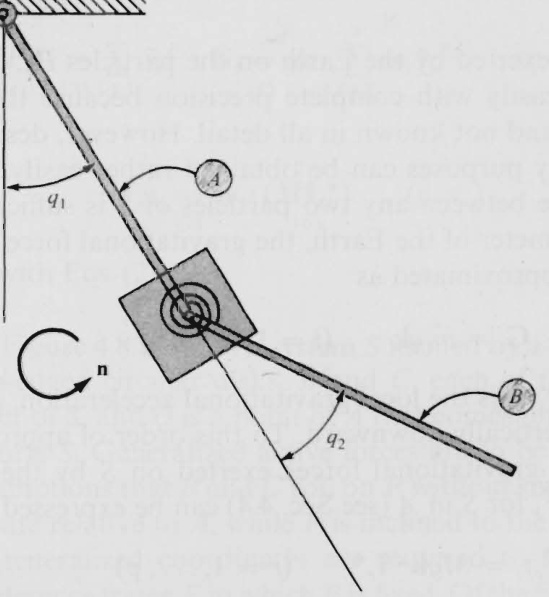
Figure 4.7.1

and let f_{r}\left(r=1,2\right) be the contribution of the spring and damper forces to the generalizedactiveforce \boldsymbol{F}_{r} (r=1,2) .Then

f_{r}\underset{(4.6\,.1)}{=}\mathbf{\omega}\mathbf{o}_{r}^{\,A}\cdot\mathbf{T}_{A}\,+\,\mathbf{o}_{r}^{\,B}\cdot\mathbf{T}_{B}\qquad(r=1,2)

Now,

\begin{array}{l}{{{\bf{\dot{o}}}^{A}={\dot{q}}_{1}{\bf{n}}=u_{1}{\bf{n}}}}\\ {{\mathrm{\boldmath~\Lambda~}}}\\ {{{\bf{\dot{o}}}^{B}=({\dot{q}}_{1}+{\dot{q}}_{2}){\bf{n}}=(u_{1}+u_{2}){\bf{n}}}}\end{array}

so that

\begin{array}{r}{\pmb{\omega_{1}}^{A}=\pmb{\mathrm{~n~}}\qquad\pmb{\omega_{2}}^{A}=0\qquad\pmb{\omega_{1}}^{B}=\pmb{\mathrm{~n~}}\qquad\pmb{\omega_{2}}^{B}=\pmb{\mathrm{~n~}}}\\ {\mathrm{(5)}\qquad\qquad\qquad\mathrm{(5)}\qquad\qquad\qquad\mathrm{(6)}\qquad\qquad\qquad\mathrm{(6)}}\end{array}

Hence.

\begin{array}{r}{f_{1}=\textbf{n}\cdot\mathbf{T}_{A}+\textbf{n}\cdot(-\mathbf{T}_{A})=0}\\ {\quad\quad(4)\ (7)\quad\quad\quad\quad(7)\quad\quad\quad(2)}\end{array}

and

\begin{array}{c}{{f_{2}=\mathrm{\bf~0}\cdot{\bf T}_{A}+{\bf n}\cdot(-{\bf T}_{A})=\mathrm{\bf~-(}\sigma q_{2}\mathrm{\bf~+~}\delta\dot{q}_{2})}}\\ {{\mathrm{\bf~\Sigma~}_{\{4\}}\mathrm{\bf~\Sigma}(\tau)\qquad\qquad\qquad\mathrm{\bf~\Sigma}_{\{2\}}\mathrm{\bf~\;\;}}}\end{array}

Thus, the interaction forces associated with the spring and damper here contributeto F_{2} but not to F_{1} The reader should verify that,if u_{1} and u_{2} are defined as u_{1}=\dot{q}_{1} u_{2}=\dot{q}_{1}+\dot{q}_{2} , rather than as in Eqs. (3),then the spring forces and damper forces contribute to both F_{\scriptscriptstyle1} and F_{2}

4.8 TERRESTRIAL GRAVITATIONAL FORCES

The gravitational forces exerted by the Earth on the particles P_{1},\dots,P_{v} of aset S cannot be evaluated easily with complete precision because the constitution of the Earth is complex and not known in all detail. However, descriptions sufficiently accurate for many purposes can be obtained rather easily. For example, when the largest distance between any two particles of s is sufficiently small in comparison with the diameter of the Earth, the gravitational force \mathbf{G}_{i} exerted on P_{i} by the Earth can be approximated as

\mathbf{G}_{i}=m_{i}g\mathbf{k}\qquad(i=1,\ldots,\nu)

where m_{i} is the mass of P_{i},g is the local gravitational acceleration, and \mathbf{k} is a unit vector locally directed vertically downward. To this order of approximation, the contribution (\widetilde{F}_{r})_{;} of all gravitational forces exerted on s by theEarth to the generalized active force {\widetilde{F}}_{\nu} for s in A (see Sec. 4.4) can be expressed as

(\widetilde{F}_{r})_{\gamma}=M g\mathbf{k}\cdot\widetilde{\mathbf{v}}_{r}^{\ \ast}\qquad(r=1,\ldots,p)

where M is the total mass of s and \tilde{\mathbf{v}}_{r}^{\ast} is the rth partial velocity of the mass center of s in A

As an alternative to using Eqs. (2), one can deal with P_{1},\dots,P_{v} individually by expressing (\widetilde{F}_{r})_{\widetilde{\gamma}} as

(\widetilde{F}_{r})_{\?\gamma}=\sum_{i\,=\,1}^{\nu}\,\widetilde{\mathbf{v}}_{r}^{\,\,P_{i}}\cdot{\mathbf{G}}_{i}\qquad(r=1,\ldots,p)

Whether it is more convenient to use Eqs. (2) or Eqs. (3) depends on the relative easeoffinding \tilde{\mathbf{v}}_{r}^{\mathrm{~*~}}(r=1,\dots,p) , on the one hand, and \tilde{\Psi}_{r}^{~P_{i}}~(r=1,\,\cdot\,.\,.\,,\,p;\,i= 1,\ldots,\nu) , on the other hand.

Derivation The position vector \boldsymbol{\mathbf{p}}^{*} from a point o fixed in _{A} to the mass center of s is related to the position vectors \mathfrak{p}_{1},\,.\,.\,.\,.\,\mathfrak{p}_{\mathrm{v}} from o to the particles of s by

M\mathbf{p}^{*}\underset{(3.1.2)}{=}\sum_{i=1}^{v}m_{i}\mathbf{p}_{i}

Differentiation with respect to t in A yields

M\mathbf{v}^{*}=\sum_{i=1}^{\nu}\ m_{i}\mathbf{v}^{P_{i}}

Consequently, the partial velocities \tilde{\mathbf{v}}_{r}^{\ *} and \tilde{\mathbf{v}}_{r}{}^{P_{i}}\left(r=1,\dots,p\right) are related to each other by [see Eq. (2.14.4)]

M\tilde{\Psi}_{r}{}^{*}=\sum_{(5)\;i=1}^{\nu}m_{i}\,\tilde{\Psi}_{r}{}^{P_{i}}\qquad(r=1,\ldots,p)

Now,

(\widetilde{F}_{r})_{\gamma}=\sum_{(3)}^{\nu}\widetilde{\mathbf{v}}_{r}^{\,P_{i}}\cdot{\mathbf{G}}_{i}=g\mathbf{k}\cdot\sum_{i=1}^{\nu}m_{i}\widetilde{\mathbf{v}}_{r}^{\,P_{i}}\qquad(r=1,\ldots,p)

Hence,

(\Tilde{F}_{r})_{\gamma}=g\mathbf{k}\cdot(M\Tilde{\mathbf{v}}_{r}^{\ast})\qquad(r=1,\ldots,p)

in agreerment with Eqs. (2).

ExampleFigure 4.8.1 shows a system s formed by a rigidframe A that carries two sharp-edged circular disks, B and C ,each of radius R .Point S^{*} is the mass center of s , and Q is a point of A that comes into contact with a plane P that supports S. Generalized active forces are to be determined on the basis of the assumptions that B and C roll on P without slipping and are completely free torotaterelative to A ,while P is inclined to the horizontal at an angle \theta

Five generalized coordinates are required to specify the configuration of s in areferenceframe F in which P is fixed. Of thefive associated generalized speeds, three are dependent on the remaining two when B and \textrm{C} roll on P withoutslipping.Inotherwords,if \boldsymbol{u}_{1} and u_{2} aredefinedas

u_{1}\triangleq\mathbf{\omega}\bullet\cdot\mathbf{a}_{1}\qquad u_{2}\triangleq\mathbf{v}^{D}\cdot\mathbf{a}_{2}

where {\bf a}_{1} and {\mathbf a}_{2} are unit vectors directed as shown in Fig. 4.8.1, \mathbf{o}^{A} is the angular velocity of A in F and \mathbf{v}^{D} is the velocity in F of the midpoint D of the axle that carries B and C , then the velocity in F of every point of s can be

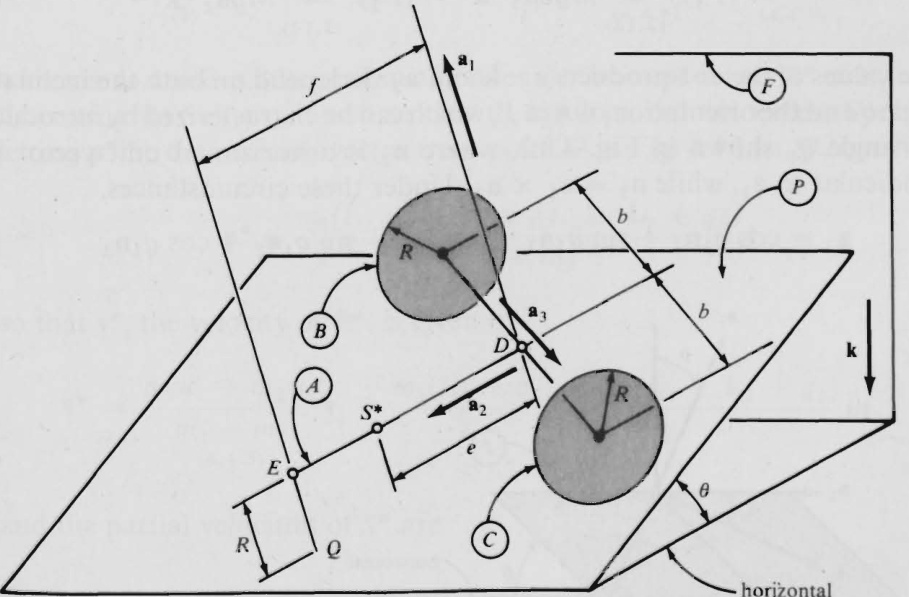
Figure 4.8.1

expressed as a linear function of u_{1} and u_{2} . For example, \mathbf{v}^{*} ,the velocity of S^{*} in \boldsymbol{\dot{F}} ,becomes (see Fig. 4.8.1 for {\mathbf{a}}_{3}

\begin{array}{r}{\mathbf{v}^{*}\ \ \ =\ u_{2}\,\mathbf{a}_{2}\,+\,e u_{1}\mathbf{a}_{3}}\\ {(2,7.1)}\end{array}

and \mathbf{v}^{Q} ,the velocity in F of thepoint \boldsymbol{Q} of A that comes into contact with A ,is

\begin{array}{r}{\mathbf{v}^{Q}\quad=\quad u_{2}\,\mathbf{a}_{2}\,+\,f u_{1}\mathbf{a}_{3}}\\ {(2.7,1)\quad\quad\quad\quad\quad\quad}\end{array}

The associated partial velocities are

\begin{array}{r l}{\tilde{\mathbf{v}}_{1}^{~*}=~e\mathbf{a}_{3}}&{\qquad\tilde{\mathbf{v}}_{2}^{~*}=~\mathbf{a}_{2}}\\ {{\scriptstyle(10)}}&{}\\ {\tilde{\mathbf{v}}_{1}^{~Q}=~f\mathbf{a}_{3}}&{\qquad\tilde{\mathbf{v}}_{2}^{~Q}=~\mathbf{a}_{2}}\\ {{\scriptstyle(11)}}&{}\end{array}

The only contact force that contributes to the generalized active forces \tilde{F}_{1} and \tilde{F}_{2} is (seeSec.4.5) theforce exerted on A by P at Q Whenthisforceis represented as Q_{1}\mathbf{a}_{1}+Q_{2}\mathbf{a}_{2}+Q_{3}\mathbf{a}_{3} ,then (\widetilde{F}_{r})_{Q} ,itscontributionto \tilde{F}_{r} ,is given by

(\tilde{F}_{r})_{Q}=\tilde{\bf v}_{r}^{~Q}\cdot(Q_{1}{\bf a}_{1}^{~}+Q_{2}{\bf a}_{2}^{~}+Q_{3}{\bf a}_{3}^{~})\qquad(r=1,2)

so that

(\widetilde{F}_{1})_{Q}\!\!\!\!\!\!\!\!=\!\!\!\!\!\!\!\!\!\!\!\!\!\!\!\!\!\!\!\!\!\!\!\!\!\!\!\!\!\!\!\!\!\!\!\!\!\!\!\!(\widetilde{F}_{2})_{Q}\!\!\!\!\!\!\!\!\!\!\!\!\!(\widetilde{F}_{3,14})\!\!\!\!\!\!\!\!\!\!\!\!\!\!\!\!\!\!\!\!\!\!\!\!\!\!\!\!\!\!\!\!\!\!\!\!\!\!\!\!\!\!\!\!\!\!\!\!\!\!\!\!\!\!\!\!\!\!\!\!\!\!\!\!\!\!\!\!\!\!\!\!\!\!\!\!\!\!\!\!\!\!\!\!\!\!\!\!\!\!\!\!\!\!\!\!\!\!\!\!\!\!\!\!\!\!\!\!\!\!\!\!\!\!\!\!\!\!\!\!\!\!\!\!\!\!\!\!\!\!\!\!\!\!\!\!\!\!\!\!\!\!\!\!\!\!\!\!\!\!\!\!\!\!\!\!\!\!\!\!\!\!\!\!\!\!\!\!\!\!\!\!\!\!\!\!\!\!\!\!\!\!\!\!\!\!\!\!\!\!\!\!\!\!\!\!\!\!\!\!\!\!\!\!\!\!\!\!\!\!\!\!\!\!\!\!\!\!\!\!\!\!\!\!\!\!\!\!\!\!\!\!\!\!\!\!\!\!\!\!\!\!\!\!\!\!\!\!\!\!\!\!\!\!\!\!\!\!\!\!\!\!\!\!\!\!\!\!\!\!\!\!\!\!\!\!\!\!\!\!\!\!\!\!\!\!\!\!\!\!\!\!\!\!\!\!\!\!\!\!\!\!\!\!\!\!\!\!\!\!\!\!\!\!\!\!\!\!\!\!\!\!\!\!\!\!\!\!\!\!\!\!\!\!\!\!\!\!\!\!\!\!\!\!\!\!\!\!\!\!\!\!\!\!\!\!\!\!\!\!\!\!\!\!\!\!\!\!\!\!\!\!\!\!\!\!\!\!\!\!\!\!\!\!\!\!\!\!\!\!\!\!\!\!\!\!\!\!\!\!\!\!\!\!\!\!\!\!\!\!\!\!\!\!\!\!\!\!\!\!\!\!\! 

Letting M denote the mass of s wehavefor (\tilde{F}_{r})_{\gamma} ,the contribution to \widetilde{F}_{r}\left(r=1,2\right) of the gravitational forces exerted on {\cal S} by the Earth,

({\widetilde{F}}_{1})_{\gamma}\mathop{=}_{(2,12)}M g e{\mathbf{a}}_{3}\cdot\mathbf{k}\qquad({\widetilde{F}}_{2})_{\gamma}\mathop{=}_{(2,12)}M g{\mathbf{a}}_{2}\cdot\mathbf{k}

The values of the dot-products {\bf a}_{3}\cdot{\bf k} and {\bf{a}}_{2}\cdot{\bf{k}} depend on both theinclination angle \theta and the orientation of A in P which can be characterized by introducing the angle q_{1} shown in Fig.4.8.2, where \mathbf{n}_{2} is a horizontal unit vector perpendicular to {\bf a}_{1} while \mathbf{n}_{3}=\mathbf{a}_{1}\,\times\,\mathbf{n}_{2} Under these circumstances,

\mathbf{a}_{2}=\cos q_{1}\mathbf{n}_{2}+\sin q_{1}\mathbf{n}_{3}\qquad\mathbf{a}_{3}=-\sin q_{1}\mathbf{n}_{2}+\cos q_{1}\mathbf{n}_{3}

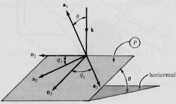
Figure 4.8.2

and

\mathbf{k}=\mathbf{-}\cos\theta\mathbf{a}_{1}+\sin\theta\mathbf{n}_{3}

Hence,

(\tilde{F}_{1})_{\gamma}\mathop{=}_{(16-18)}M g e\sin\theta\cos q_{1}\qquad(\tilde{F}_{2})_{\gamma}\mathop{=}_{(16-18)}M g\sin\theta\sin q_{1}

and the desired generalized active forces are

\tilde{F}_{1}=(\tilde{F}_{1})_{Q}+(\tilde{F}_{1})_{\gamma}\mathop{=}_{(15,19)}f Q_{3}+M g e\sin\theta\cos q_{1}

and

\tilde{F}_{2}=(\tilde{F}_{2})_{Q}+(\tilde{F}_{2})_{\gamma}\mathop{=}_{(15,19)}Q_{2}+M g\sin\theta\sin q_{1}

The reason for using Eqs. (2) rather than Eqs. (3) to find (\widetilde{F}_{1})_{\gamma} and (\widetilde{F}_{2})_{\gamma} [see Eqs. (16)] is that it would be very laborious to deal individually with each of the particles forming A,B, and C . By way of contrast, consider once again the contributions of gravitational forces to the generalized active forces F_{1} and F_{2} in the example in Sec. 4.4. Since the partial velocities of \boldsymbol{P}_{1} and P_{2} are available in Eqs. (4.4.8) and (4.4.9), (F_{\imath})_{\gamma} and (F_{2})_{\gamma} are formed easily as

\begin{array}{r l}&{(F_{1})_{\gamma}={\mathbf{v}_{1}}^{P_{1}}\cdot(m_{1}g\mathbf{k})+{\mathbf{v}_{1}}^{P_{2}}\cdot(m_{2}g\mathbf{k})=m_{1}g\cos\theta+\begin{array}{c}{0}\\ {(4.4.8)}\end{array}}\\ &{(F_{2})_{\gamma}={\mathbf{v}_{2}}^{P_{1}}\cdot(m_{1}g\mathbf{k})+{\mathbf{v}_{2}}^{P_{2}}\cdot(m_{2}g\mathbf{k})=\begin{array}{c}{0}\\ {(4.4.8)}\end{array}+m_{2}g\cos\theta}\end{array}

whereas, to use Eqs. (2), one must first locate the mass center s^{*} of \boldsymbol{P}_{1} and P_{2} ， determine its velocity, and use this to form partial velocities. Specifically, letting \mathsf{p}^{*} be the position vector from point o in Fig. 4.4.1 to s^{*} , one has

\mathbf{p}^{*}=\frac{m_{1}(L_{1}+q_{1})+m_{2}(L_{1}+L_{2}+q_{2})}{m_{1}+m_{2}}\mathbf{t}_{1}

so that \mathbf{v}^{\ast} , the velocity of P^{*} , is given by

\mathbf{v^{*}}=\frac{m_{1}u_{1}+m_{2}u_{2}}{m_{1}+m_{2}}\,\mathbf{t}_{1}\,+\frac{m_{1}(L_{1}+q_{1})+m_{2}(L_{1}+L_{2}+q_{2})}{m_{1}+m_{2}}\,\dot{\theta}\mathbf{t}_{2}

and the partial velocities of s^{*} are

\mathbf{v_{1}}^{*}={\frac{m_{1}}{m_{1}\mathbf{\alpha}+m_{2}}}\mathbf{t}_{1}\qquad\mathbf{v_{2}}^{*}={\frac{m_{2}}{m_{1}\mathbf{\alpha}+m_{2}}}\mathbf{t}_{1}

Now one can refer to Eqs. (2) to write

(F_{1})_{\gamma}=[(m_{1}\,+\,m_{2})g{\bf k}]\cdot\left(\frac{m_{1}}{m_{1}\,+\,m_{2}}\,{\bf t}_{1}\right)=m_{1}g\cos\theta

(F_{2})_{\gamma}=[(m_{1}\,+\,m_{2})g{\bf k}]\cdot\left(\frac{m_{2}}{m_{1}\,+\,m_{2}}\,{\bf t}_{1}\right)=m_{2}g\cos\theta

These results agree with Eqs. (22) and (23), but more effort had to be expended to derive Eqs. (27) and (28) than to generate Eqs. (22) and (23).

4.9 BRINGING NONCONTRIBUTING FORCES INTOEVIDENCE

As was mentioned in Sec. 4.5, the fact that certain forces acting on the particles of a system make no contributions to generalized active forces usually is helpful. But it can occur that precisely such a noncontributing force, or a torque of a couple formed by noncontributing forces, is of interest in its own right. In that event, one can bring this force or torque into evidence through the introduction of a generalized speed properly related to the force or torque in question, that is, a generalized speed that gives rise to a partial velocity of the point of application of the force, or a partial angular velocity of the rigid body on which the couple acts, such that the dot-product of the partial velocity and the force, or the dotproduct of the partial angular velocity and the torque, does not vanish. The force or torque of interest then comes into evidence in the generalized active force corresponding to the additional degree of freedom associated with the additional generalizedspeed.

The introduction of a suitable additional generalized speed is accomplished by permitting points to have certain velocities, or rigid bodies to have certain angular velocities, which they cannot, in fact possess, doing so without introducing additional generalized coordinates. When forming expressions for velocities and/or angular velocities, one then takes the additional generalized speed into account, but one uses the same generalized coordinates as before, and one identifies partial velocities and partial angular velocities corresponding to the additional generalized speed by inspection, as always. The partial velocities and partial angular velocities corresponding to the original generalized speeds, as well as the associated original generalized active forces, remain unaltered.

Example In Fig. 4.9.1,P is a particle of mass m that can slide freely on a smooth, uniform rod \pmb R of mass M and length 2L,\,R is rigidly attached at an angle \beta to a light sleeve s that is supported by a smooth, fixed vertical shaft V and a smooth bearing surface \pmb{B} and s is subjected to the action of a couple whose torque T is given by

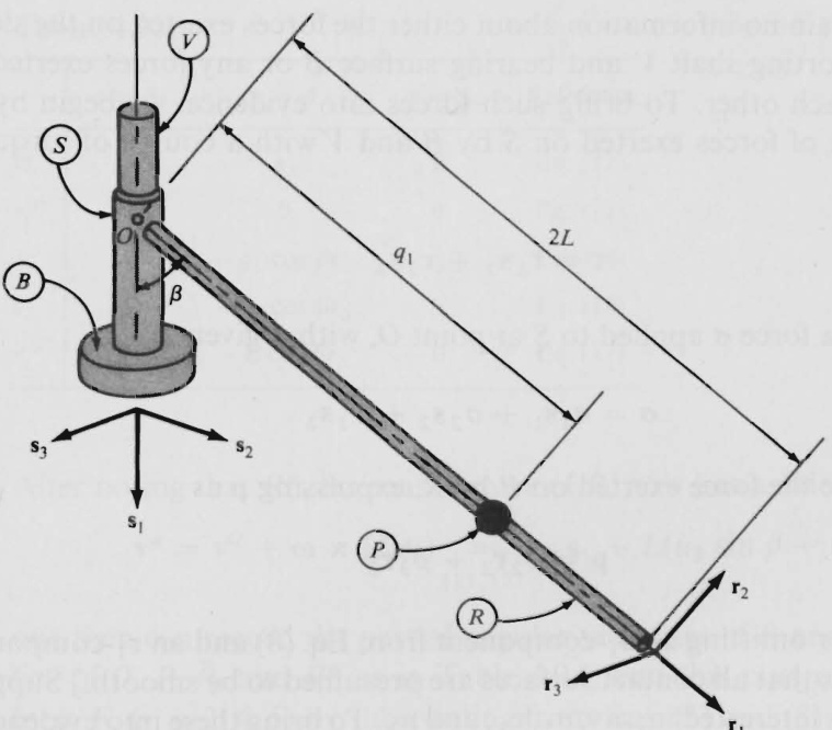
Figure 4.9.1

where T is time-dependent and \mathbf{s}_{1} is a unit vector directed vertically downward. The unit vectors {\bf s}_{2},\,{\bf s}_{3},\,{\bf r}_{1},\,{\bf r}_{2} , and {\bf r}_{3} in Fig. 4.9.1 are defined as follows: s_{2} is perpendicular to \mathbf{s}_{1} and parallel to the plane determined by the axes of s and R;\mathbf{s}_{3}=\mathbf{s}_{1}\times\mathbf{s}_{2};\mathbf{r}_{1},\mathbf{r}_{2},\mathbf{r}_{3} form a dextral set of mutually perpendicular unit vectors, with \mathbf{r}_{1} parallel to the axis of R and {\bf r}_{2} parallel to the plane determinedbytheaxesof s and R

The system formed by P,R and s possesses two degrees of freedom and. if generalized speeds \boldsymbol{\mathscr{u}}_{1} and u_{2} are defined as

u_{1}\triangleq\dot{q}_{1}\qquad u_{2}\triangleq\mathbf{o}\cdot\mathbf{s}_{1}

where q_{1} is the distance from o to P and \mathbf{\omega}_{\infty} is the angular velocity of R ,then the associated partial angular velocities of R and partial velocities of P are

\begin{array}{l l}{{{\bf{\omega}}_{1}}=0\quad}&{{\bf{\omega}}_{1}={\bf{r}}_{1}}\\ {{{\bf{\omega}}_{2}}={\bf{s}}_{1}\quad}&{{\bf{\omega}}_{{\bf{v}}_{2}}=q_{1}\sin\beta{\bf{r}}_{3}}\end{array}

Hence, the generalized active forces F_{1} and F_{2} ,found by substituting from Eqs. (1), (3), and (4) into [see Eqs. (4.6.1) and (4.8.1)]

F_{r}=\mathbf{\omega_{r}}\cdot\mathbf{T}+\mathbf{v_{r}}\cdot(m g\mathbf{s}_{1})\qquad(r=1,2)

are

\begin{array}{l}{F_{1}=m g\cos\beta}\\ {F_{2}=T}\end{array}

and these contain noinformation about either theforces exerted on the sleeve s by the supporting shaft V and bearing surface \pmb{B} or any forces exerted by \pmb{P} and \pmb R on each other. To bring such forces into evidence, we begin by replacing the set of forces exerted on S by \boldsymbol{B} and V with acouple of torque \pmb{\uptau} expressed as

{\pmb\tau}=\tau_{2}{\bf s}_{2}+\tau_{3}{\bf s}_{3}

together with a force \pmb{\upsigma} applied to s at point o ,with \pmb{\upsigma} given by

{\pmb{\sigma}}=\sigma_{1}{\bf s}_{1}\,+\,\sigma_{2}\,{\bf s}_{2}\,+\,\sigma_{3}\,{\bf s}_{3}

and we let \pmb{\uprho} be the force exerted on P by \pmb R , expressing {\pmb\uprho} as

\pmb{\uprho}=\rho_{2}\pmb{\mathrm{r}}_{2}+\rho_{3}\pmb{\mathrm{r}}_{3}

[The reason for omitting an \mathbf{s}_{1} -component from Eq. (8) and an \mathbf{r}_{1} -component from Eq. (10) is that all contact surfaces are presumed to be smooth.] Suppose now that one is interested in, say, \sigma_{1},\tau_{2} , and \rho_{3} . To bring these into evidence in expressions for generalized forces, one permits s to move in such a way that the point o , regarded as a point of \pmb R , has a velocity {\bf v}^{o} given by

\mathbf{v}^{o}=u_{3}\mathbf{s}_{1}

while R has an angular velocity \mathbf{\omega} that can be expressed as

\mathbf{\omega}\bullet=u_{2}\mathbf{s}_{1}+u_{4}\mathbf{s}_{2}

Also, one allows P to have a velocity \mathbf{v} such that \pmb{P} can lose contact with \pmb R or can penetrate \pmb R by moving in the direction of \mathbf{r}_{3} , which is accomplished by letting \overline{{\mathbf{v}}} denote the velocity of the point \bar{\pmb R} of \pmb R with which P is in contact and then writing

\begin{array}{r}{\mathbf{v}\quad=\quad\overline{{\mathbf{v}}}+\mathbf{\nabla}^{R}\mathbf{v}^{P}}\\ {(2.8.1)}\end{array}

with

\bar{\mathbf{v}}_{(2.7.1)}^{\ \ =\ \ }\mathbf{v}^{o}+\mathbf{\omega}\mathbf{e}\times(q_{1}\mathbf{r}_{1})\mathbf{\omega}_{(11,12)}^{\ \ =\ \ }u_{3}\mathbf{s}_{1}+q_{1}(u_{2}\sin\beta-u_{4}\cos\beta)\mathbf{r}_{3}

and

^R{\mathbf{v}}^{P}={\dot{q}}_{1}{\mathbf{r}}_{1}+u_{5}\,{\mathbf{r}}_{3}=u_{1}{\mathbf{r}}_{1}+u_{5}\,{\mathbf{r}}_{3}

so that

\mathbf{v}_{\phantom{}_{(13-15)}}=u_{1}\mathbf{r}_{1}+u_{2}q_{1}\sin\beta\mathbf{r}_{3}+u_{3}\mathbf{s}_{1}-u_{4}q_{1}\cos\beta\mathbf{r}_{3}+u_{5}\mathbf{r}_{3}

Table 4.9.1

<html>

	r=3	r = 4	r= 5	Reference
	0	S2	0	Eq. (12)
V.0	S1	0	0	Eq. (11)
Vr	$1	-91 cos βr3	r3	Eq. (16)
V,	$1	-91 cosβr3	0	Eq. (14)
V*	S1	-L cosβr3	0	Eq. (17)

</html>

After noting that R^{*} , the mass center of \pmb R , now has a velocity \mathbf{v^{*}} given by

\mathbf{v^{*}}=\mathbf{v}^{o}+\mathbf{\upomega}\times(L\mathbf{r}_{1})\mathbf{\Pi}_{(11,12)}=u_{3}\mathbf{s}_{1}+L(u_{2}\sin\beta-u_{4}\cos\beta)\mathbf{r}_{3}

one then can record the partial angular velocities of \pmb R and the partial velocities of O,P,{\bar{R}} ,and R^{*} as in Table 4.9.1, and this puts one into position to form F_{\mathrm{,}} (r=3,4,5) by substituting from Eqs. (1) and (8)-(10) into

\begin{array}{r}{F_{r}=\mathbf{\upomega}_{r}\cdot(\mathbf{T}+\boldsymbol{\uptau})+\mathbf{\upv}_{r}^{\,o}\cdot\mathbf{\upsigma}+\mathbf{\upv}_{r}\cdot(m g\mathbf{s}_{1}+\mathbf{\uprho})\quad\quad}\\ {+\ \overline{{\mathbf{v}}}_{r}\cdot(-\mathbf{\uprho})+\mathbf{\upv}_{r}^{\,*}\cdot(M g\mathbf{s}_{1})\quad\quad(r=3,4,5)}\end{array}

which leads to

\begin{array}{l}{{F_{3}=\sigma_{1}+(m+M)g}}\\ {{{}}}\\ {{F_{4}=\tau_{2}}}\\ {{{}}}\\ {{{}F_{5}=\rho_{3}}}\end{array}

The quantities \sigma_{2},\sigma_{3},\tau_{3} , and \rho_{2} , which are absent from F_{1},\ldots,F_{5} , can be brought into evidence similarly; that is, if u_{6},\ldots,u_{9} are introduced such that

\begin{array}{r}{\mathbf{v}^{o}=u_{3}\mathbf{s}_{1}+u_{6}\mathbf{s}_{2}+u_{7}\mathbf{s}_{3}}\\ {\mathbf{\omega}=u_{2}\mathbf{s}_{1}+u_{4}\mathbf{s}_{2}+u_{8}\mathbf{s}_{3}}\end{array}

and

^R_{\mathbf{\overline{{\Psi}}}}P=u_{1}\mathbf{r}_{1}+u_{9}\mathbf{r}_{2}+u_{5}\mathbf{r}_{3}

then the generalized active forces corresponding to u_{6},\ldots,u_{9} are

\begin{array}{l}{{F_{6}=\sigma_{2}}}\\ {{F_{7}=\sigma_{3}}}\\ {{F_{8}=\tau_{3}-(m q_{1}+M L)g\sin\beta}}\\ {{F_{9}=\rho_{2}-m g\sin\beta}}\end{array}

4.10 COULOMB FRICTION FORCES

Suppose that a particle P or a rigid body B belonging to a simple nonholonomic system S possessing p degrees of freedom in a reference frame \pmb{A} (see Sec. 2.13) is in contact with a rigid body C (which may, or may not, belong to s ). Then, if P or \textbf{\emph{B}} is sliding on C ,the contributions of contact forces exerted on P or \pmb{B} by c to the generalized active forces F_{1},\ldots,F_{p} (see Sec. 4.4) depend on both the magnitudes and the directions of such contact forces. When contact takes place across dry, clean surfaces, certain information regarding the magnitudes and the directions of contact forces can be obtained from the laws of Coulomb friction, which will now be stated.

When a particle P that is in contact with a rigid body C is at rest relative to C then C exerts on P a contact force C that can be expressed as

\mathbf{C}=N\mathbf{v}+\,T\pmb{\uptau}

where \pmb{\nu} is a unit vector normal to the surface \Sigma of C at P and directed from C toward P,\tau is a unit vector perpendicular to \mathbf{v},N is non-negative, and T satisfies the inequality

\vert\,T\vert\leq\mu N

in which \pmb{\mu} , called the coefficient of static friction for P and C ,is a quantity whose value depends solely on the materials of which P and _{C} are made. Typical values are 0.2 for metal on metal, 0.6 for metal on wood.

When P is in a state of impending tangential motion relative to c that is,when P is on the verge of moving tangentially relative to C then

\vert\,T\,\vert\,=\,\mu N

andthevector T\tau appearing in Eq. (1) points in the direction opposite to that in which P is about to move relative to C

When P is sliding relative to C , Eq. (1) remains in force, but the inequality (2) gives way to the equality

\vert\,T\vert=\mu^{\prime}N

where \mu^{\prime} , called the coefficient of kinetic friction for P and C , has a value generally smaller than that of \pmb{\mu} ; and the vector T\tau in Eq. (1) now is directed oppositely to CvP, the velocity of P in C.

When a rigid body \pmb{B} rather than a particle P , is in contact with C , the same laws apply if the surface \pmb{\Sigma} over which B and C are in contact has an area so small that \Sigma can be regarded as a point. Otherwise, that is, when \Sigma has an area that cannot be regarded as negligibly small, the laws already stated apply in connection with every_differential element of \Sigma . More specifically, if P is a point of \pmb{B} within a portion \overline{{\Sigma}} of \boldsymbol{\Sigma} that has an area \bar{\pmb{A}} then the set of contact forces exerted on \textbf{\emph{B}} by c across \overline{{\Sigma}} can be replaced with a couple of torque \mathbf{M} together with a force \mathbf{c} whose line of action passes through \pmb{P};\mathbf{M} and \mathbf{c} depend on \pmb{\bar{A}} , and both approach zero as \bar{A} approaches zero, but

\operatorname*{lim}_{\bar{\boldsymbol{A}}\rightarrow0}\frac{\mathbf{M}}{\bar{\boldsymbol{A}}}=0

whereas \mathbf{C}/\overline{{A}} has a nonzero limit that can be expressed as

\operatorname*{lim}_{\bar{A}\to0}\frac{\mathbf{C}}{\overline{{A}}}=n\mathbf{v}+t\bar{\mathbf{\tau}}

where \pmb{n}_{i} called the pressure at point P_{s} and \boldsymbol{t} , called the shear at P , depend on the position of \pmb{P} within \Sigma,n is non-negative, and \pmb{\nu} and \pmb{\uptau} have the same meanings as before. Equations (5) and (6) imply that, if P is a point of \boldsymbol{B} lying within a differential element \pmb{d}\pmb{\Sigma} of \Sigma having an area d A , the set of contact forces exerted on \pmb{B} by c across \pmb{d}\pmb{\Sigma} is equivalent to a force \scriptstyle d\mathbf{C} whose line of action passes through \pmb{P} and that is given by

d\pmb{\ C}=\left(n\pmb{\nu}+t\pmb{\tau}\right)d A

This equation takes the place of Eq. (1) when \boldsymbol{B} and C are in contact over an extended surface, and the relationships (2)-(4) then are replaced with, respectively,

|t|\leq\mu n

when P is at rest relative to C

|t|=\mu n

when P is in a state of impending tangential motion relative to C and

\vert t\vert=\mu^{\prime}n

when \pmb{P} is sliding relative to c

When a particle P is in contact with a rigid body c modeled as matter distributed along a curve \Gamma (for example, a thin rod modeled as matter distributed along a straight line), then Eqs. (1)-(4) and the statements made in connection with these equations remain in force, provided that \pmb{\uptau} is regarded as a unit vector tangent to \Gamma at P while \pmb{\nu} is simply a unit vector perpendicular to t. Similarly, when contact between two rigid bodies \pmb{B} and c is regarded as taking place along a curve \Gamma (for example, when a generator of a right-circular cylinder is in contact with a plane), then Eq. (7) applies after d A has been replaced with \pmb{d L} , the length of a differential element d\Gamma of \Gamma and \pmb{\nu} and \pmb{\uptau} then have their original meanings.

Example Considering once again the system formed by the sleeve S, rod \pmb R ， and particle P depicted in Fig. 4.9.1 and considered previously in the example in Sec. 4.9, suppose that the contact between S and the bearing surface \pmb{B}_{\pmb{\cdot}} as well as that between P and \pmb R , takes place across a rough, rather than a smooth, surface, but that the vertical shaft V can be regarded as smooth, as heretofore. Then, when S is moving relative to \textbf{\emph{B}} , and P relative to \pmb R , contact forces that contribute to the generalized active forces F_{1} and F_{2} comeinto play. (F_{r})_{c} , the contribution to F (r=1,2) of the contact forces, will now be determined.

The contact force p exerted by R on P can be expressed as

\mathbf{\uprho}=\rho_{1}\mathbf{r}_{1}+\rho_{2}\mathbf{r}_{2}+\rho_{3}\mathbf{r}_{3}

and the contact force \bar{\pmb{\uprho}} exerted by P on R is given by

{\bar{\mathfrak{p}}}=-\,\mathfrak{p}

Hence, letting \overline{{\mathbf{v}}}_{r} (r=1,2) denote the partial velocities of the point of \pmb R at which \bar{\pmb{\uprho}} is applied to R , so that

\begin{array}{r l r}{\overline{{\mathbf{v}}}_{1}=0}&{{}}&{\overline{{\mathbf{v}}}_{2}=q_{1}\,\sin\,\beta\mathbf{r}_{3}}\end{array}

one can express the contributions of {\pmb\uprho} and \bar{\pmb{\uprho}} to the generalized active forces F_{1} as

\begin{array}{r}{\mathbf{v}_{1}\cdot\mathbf{\uprho}+\bar{\mathbf{v}}_{1}\cdot\bar{\mathbf{p}}\ =\ \underset{(4.9.3)}{\mathbf{r}}\cdot\ \mathbf{\uprho}\ +\ 0\ \ =\ \rho_{1}}\end{array}

and

\begin{array}{r}{\mathbf{v}_{2}\cdot\mathbf{\uprho}+\overline{{\mathbf{v}}}_{2}\cdot\overline{{\mathbf{\uprho}}}=(\mathbf{v}_{2}-\overline{{\mathbf{v}}}_{2})\cdot\mathbf{\uprho}\qquad=\qquad0}\\ {\qquad\qquad\qquad\qquad\qquad(4.9.4,13)}\end{array}

The laws of friction make it possible to express \rho_{1} in terms of \rho_{2} and \rho_{3} for \rho_{1}\mathbf{r}_{1} in Eq. (11) corresponds to the second term of Eq. (1) while \rho_{2}\,\mathbf{r}_{2}+\rho_{3}\,\mathbf{r}_{3} plays the part of the first term. Accordingly,

|\rho_{1}|=\mu_{1}{}^{\prime}(\rho_{2}{}^{2}\ +\ \rho_{3}{}^{2})^{1/2}

where \mu_{1}{'} is the coefficient of kinetic friction _for P and \pmb R .Furthermore, \rho_{1}\mathbf{r}_{1} must have a direction opposite to that of \pmb{R_{\mathbf{v}}^{P}} , the velocity of P in \pmb R , which means that \rho_{1}\mathbf{r}_{1} can be written

\begin{array}{r l}&{\rho_{1}\mathbf{r}_{1}=\mathbf{\phi}-\vert\rho_{1}\vert\frac{^{R}\mathbf{v}^{P}}{\vert^{R}\mathbf{v}^{P}\vert}=\mathbf{\phi}-\mu_{1}^{\prime}(\rho_{2}^{\mathbf{\phi}_{2}^{2}}+\rho_{3}^{\mathbf{\phi}_{2}^{2}})^{1/2}\frac{u_{1}\mathbf{r}_{1}}{\vert u_{1}\vert}}\\ &{\qquad\qquad=\mathbf{\phi}-\mu_{1}^{\prime}(\rho_{2}^{\mathbf{\phi}_{2}^{2}}+\rho_{3}^{\mathbf{\phi}_{2}^{2}})^{1/2}\:\mathrm{sgn}\;u_{1}\mathbf{r}_{1}}\end{array}

from which it follows that

\rho_{1}=\,-\mu_{1}^{\;\prime}({\rho_{2}}^{2}+{\rho_{3}}^{2})^{1/2}\;\mathrm{sgn}\;u_{1}

so that

\mathbf{v_{1}}\cdot\mathbf{\mathfrak{p}}+\bar{\mathbf{v}}_{1}\cdot\bar{\mathbf{\mathfrak{p}}}\ {\underset{(14,18)}{=}}-{\mu_{1}}^{\prime}({\rho_{2}}^{2}+{\rho_{3}}^{2})^{1/2}\operatorname{sgn}u_{1}

To deal with the contributions to \boldsymbol{F}_{1} and F_{2} of the contact forces exerted on s by \pmb{B} , we let b_{1} and b_{2} be the inner and outer radii of s , respectively, and consider ageneric differentialelement d\Sigma of the surface \Sigma of \boldsymbol{\cal S} that is in contact with B d\Sigma having the dimensions indicated in Fig.4.10.1, where \theta and z are variables used tolocate one corner, \boldsymbol{Q} ,of d\Sigma The force d\mathbf{\sigma}_{\mathfrak{O}} exertedon {\cal S} by B across d\Sigma thencanbewritten

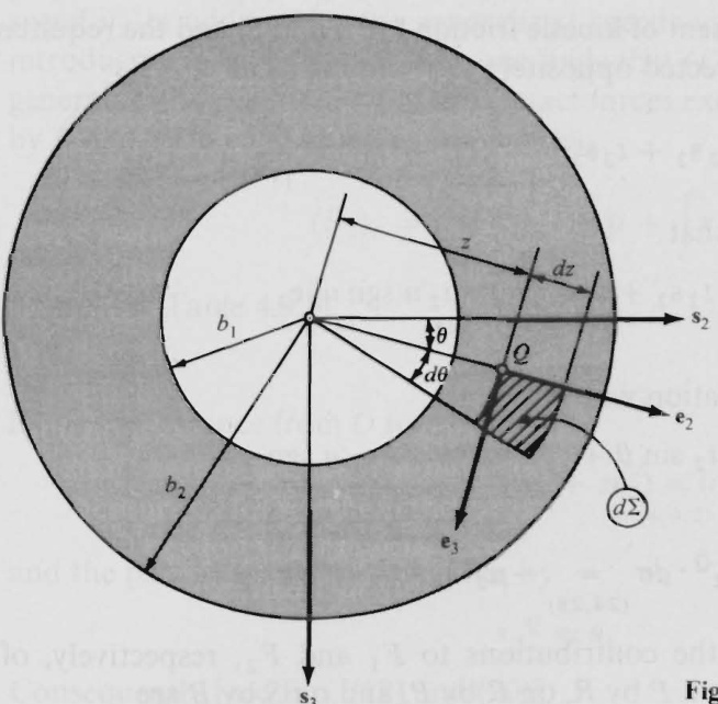
Figure 4.10.1

d\pmb{\sigma}=(-n\pmb{\mathscr{s}}_{1}+t_{2}\,\pmb{\mathscr{s}}_{2}+t_{3}\,\pmb{\mathscr{s}}_{3})\,z\,d z\,d\theta

where -\mathbf{s}_{1} ,which points from B toward S corresponds to \nu in Eq.(7) since \varrho is a point of d\Sigma , and \mathbf{v}^{Q} the velocity of \boldsymbol{Q} is given by (see Fig. 4.10.1 for the unitvectors \mathbf{e}_{2} and \mathbf{e}_{3}

{\mathfrak{v}}^{Q}={\mathfrak{o}}\times(z{\mathfrak{e}}_{2})={(u_{2}{\mathfrak{s}}_{1})}\times(z{\mathfrak{e}}_{2})=u_{2}\,z{\mathfrak{e}}_{3}

so that the partial velocities of Q are

\mathbf{v}_{1}{}^{Q}=0\qquad\mathbf{v}_{2}{}^{Q}=z\mathbf{e}_{3}

We can now express the contributions of d\mathbf{\sigma}^{\sigma} to F_{1} and F_{2} as

\mathbf{v}_{1}\mathbf{^{Q}}\cdot d\mathbf{\sigma}=\mathbf{\sigma}0

and

\begin{array}{r}{\begin{array}{r l}{\mathbf{v}_{2}^{~Q}\cdot d\mathbf{\sigma}~~=~~}&{{}\!\!z^{2}(-t_{2}\sin\theta+t_{3}\cos\theta)\,d z\,d\theta}\end{array}}\end{array}

In addition, we have the relationship

({t_{2}}^{2}+{t_{3}}^{2})^{1/2}=\mu_{2}{}^{\prime}n

where \mu_{2}{'} is the coefficient of kinetic friction for \pmb{B} and s and the requirement that t_{2}\mathbf{s}_{2}+t_{3}\mathbf{s}_{3} be directed oppositely to \mathbf{v}^{Q} implies that

t_{2}\mathbf{s}_{2}\,+\,t_{3}\mathbf{s}_{3}\,=\,-({t_{2}}^{2}+\,{t_{3}}^{2})^{1/2}\,\frac{\mathbf{v}^{Q}}{|\mathbf{v}^{Q}|}

from which it follows that

t_{2}\mathbf{s}_{2}+t_{3}\mathbf{s}_{3}\,=\,-\mu_{2}^{\,\prime}n\,\operatorname{sgn}\,u_{2}\mathbf{e}_{3}

or, upon dot-multiplication with {\mathfrak{e}}_{3} , that

-t_{2}\,\sin\,\theta\,+\,t_{3}\,\cos\,\theta\,=\,-\,\mu_{2}^{\,\prime}n\,\operatorname{sgn}\,u_{2}

Hence,

\begin{array}{r}{{\bf v}_{2}^{\ \ Q}\cdot d{\bf\sigma}_{(24,28)}=\mathrm{~\Gamma~}-\mu_{2}^{\ \prime}\ \mathrm{sgn}\ u_{2}n z^{2}\ d z\ d\theta}\end{array}

(F_{1})_{c} and (F_{2})_{c} , the contributions to F_{1} and F_{2} , respectively, of the contact forces exerted on \pmb{P} by \pmb R on \pmb R by P , and on s by \pmb{B} are

\begin{array}{r l r}{(F_{1})_{c}}&{=}&{\mathbf{v}_{1}\cdot\mathbf{\mathfrak{p}}+\bar{\mathbf{v}}_{1}\cdot\bar{\mathbf{p}}+\displaystyle\int\mathbf{v}_{1}^{\mathbf{\Omega}}\mathbf{\mathfrak{d}}\mathbf{\mathfrak{s}}\,d\mathbf{\mathfrak{q}}}\\ &{}&{=}&{-\mu_{1}^{\mathbf{\Omega}}({\rho_{2}}^{2}+\rho_{3}^{\mathbf{\Omega}}^{2})^{1/2}\mathrm{~sgn~}u_{1}}\\ &{}&{\phantom{=},\cdots\,\mu_{1}^{\mathbf{\Omega}}({\rho_{2}}^{2}+\rho_{3}^{\mathbf{\Omega}}^{2})^{1/2}\mathrm{~sgn~}u_{1}}\end{array}

and

\begin{array}{r c l}{{(F_{2})_{C}}}&{{=}}&{{{\bf v}_{2}\cdot{\bf\sigma}\mathfrak{p}+\overline{{{\bf v}}}_{2}\cdot{\bf\0}+\displaystyle\int_{{\bf v}_{2}}\!\!\!\!\!\!\!\!\!\!\!\!\!\!\!\!\!\!\!\!\!\!\!\!\!\!\!\!\!\!\!\!\!\!\!\!\!\!\!\!\!\!\!\!\!\!\!\!\!\!\!\!\!\!\!\!\!\!\!\!\!\!\!\!\!\!\!\!\!\!\!\!\!\!\!\!\!\!\!\!\!\!\!\!\!\!\!\!\!\!\!\!\!\!\!\!\!\!\!\!\!\!\!\!\!\!\!\!\!\!\!\!\!\!\!\!\!\!\!\!\!\!\!\!\!\!\!\!\!\!\!\!\!\!\!\!\!\!\!\!\!\!\!\!\!\!\!\!\!\!\!\!\!\!\!\!\!\!\!\!\!\!\!\!\!\!\!\!\!\!\!\!\!\!\!\!\!\!\!\!\!\!\!\!\!\!\!\!\!\!\!\!\!\!\!\!\!\!\!\!\!\!\!\!\!\!\!\!\!\!\!\!\!\!\!\!\!\!\!\!\!\!\!\!\!\!\!\!\!\!\!\!\!\!\!\!\!\!\!\!\!\!\!\!\!\!\!\!\!\!\!\!\!\!\!\!\!\!\!\!\!\!\!\!\!\!\!\!\!\!\!\!\!\!\!\!\!\!\!\!\!\!\!\!\!\!\!\!\!\!\!\!\!\!\!\!\!\!\!\!\!\!\!\!\!\!\!\!\!\!\!\!\!\!\!\!\!\!\!\!\!\!\!\!\!\!\!\!\!\!\!\!\!\!\!\!\!\!\!\!\!\!\!\!\!\!\!\!\!\!\!\!\!\!\!\!\!\!\!\!\!\!\!\!\!\!\!\!\!\!\!\!\!\!\!\!\!\!\!\!\!\!\!\!\!\!\!\!\!\!\!\!\!\!\!\!\!\!\!\!\!\!\!\!\!\!\!\!\!\!\!\!\!\!\!\!\!\!\!\!\!\!\!\!\!\!\!\!\!\!\!\!\!\!\!\!\!\!\!\!\!\!\!\!\!\!\!\!\!\!\!\!\!\!\!\

The definite integral in Eq. (31) can be evaluated only when the pressure \pmb{n} is known as a function of \boldsymbol{z} and \theta. To discover this functional relationship, one must use the methods of the theory of elasticity. However, satisfactory results often can be obtained in this sort of situation by making a relatively simple assumption regarding the pressure distribution in question, such as, for example, that \pmb{n} is independent of \boldsymbol{z} and \theta and thus has a value n^{*} that depends solely on the time t. Under these circumstances,

\begin{array}{c}{{(F_{2})_{C}\displaystyle=\ -\,{\mu_{2}}^{\ast}\operatorname{sgn}\,u_{2}n^{\ast}\displaystyle\int_{0}^{2\pi}\displaystyle\int_{b_{1}}^{b_{2}}\!z^{2}\,d z\,d\theta}}\\ {{\mathrm{}}}\\ {{\displaystyle=\ -\ \frac{2\pi n^{\ast}}{3}\,(b_{2}^{\,3}-b_{1}^{\,3}){\mu_{2}}^{\prime}\operatorname{sgn}\,u_{2}}}\end{array}

As will be seen later, n^{\ast} ultimately can be determined by resorting to the procedure employed in Sec. 4.9, that is, by introducing a suitable generalized speed \pmb{u}_{3} in addition to the generalized speeds u_{1} and u_{2} . Specifically, after introducing \boldsymbol{u}_{3} as in Eq. (4.9.11), one finds that (F_{3})_{C} , the contribution to the generalized active force F_{3} of all contact forces exerted by \boldsymbol{B} and V on s , and by R and P on each other, can be written

(F_{3})_{C}={\bf v}_{3}\cdot{\bf\bar{p}}+\,\overline{{{\bf v}}}_{3}\cdot\bar{{\bf p}}+\int_{}{\bf v}_{3}{\bf\mathcal{Q}}\cdot d{\bf\sigma}

where (see Table 4.9.1)

\mathbf{v}_{3}=\overline{{\mathbf{v}}}_{3}

If h is the distance from o to \Sigma , then

\begin{array}{r}{\begin{array}{c}{\mathbf{v}^{Q}\quad=\quad\mathbf{v}^{O}+\mathbf{\omega}\times(h\mathbf{s}_{1}\,+\,z\mathbf{e}_{2})=u_{3}\mathbf{s}_{1}+u_{2}z\mathbf{e}_{3}}\\ {\quad\mathbf{\omega}_{(2.7,1)}^{(2.7,1)}}\end{array}}\end{array}

and the partial velocity \mathbf{v}_{3}^{\textit{Q}} is given by

\mathbf{v}_{3}{}^{Q}=\mathbf{s}_{1}

Consequently [see Eqs. (12) and (20)],

\begin{array}{r l r}{\lefteqn{(F_{3})_{C}\qquad=}}&{{}-n^{*}\int_{0}^{2\pi}\int_{b_{1}}^{b_{2}}\!z\;d z\;d\theta}\\ {\quad}&{{}=}&{-\pi n^{*}({b_{2}}^{2}-{b_{1}}^{2})}\end{array}

The quantities \rho_{2} and \rho_{3} appearing in Eq. (30) come into evidence also when one forms the contributions (F_{5})_{C} and (F_{9})_{C} of contact forces to the generalized active forces F_{5} and F_{9} corresponding to \pmb{u_{5}} and \pmb{u_{9}} , respectively, where \pmb{u}_{5} and u_{9} have the same meaning as in Eq. (4.9.24). Specifically, in in agreement with Eqs. (4.9.21) and (4.9.28),

(F_{5})_{C}=\rho_{3}\qquad(F_{9})_{C}=\rho_{2}

Expressions for the contributions to F_{r} (r=1,2,3,5,9) of all gravitational forces acting on S,R ,and P and of the torque T described by Eq. (4.9.1) can be formulated as they were in connection with Eqs. (4.9.6), (4.9.7), (4.9.19), (4.9.21), and (4.9.28). Hence, the complete generalized active forces are

\begin{array}{l}{{F_{1}=\displaystyle m g\cos\beta-\mu_{1}^{\prime}(\rho_{2}^{2}+\rho_{3}^{2})^{1/2}\mathrm{~sgn~}u_{1}}}\\ {{\ \ \ \ (4.9,6)}}\\ {{\displaystyle F_{2}=\ {\cal T}_{-}-\frac{2\pi n^{*}}{3}(b_{2}^{3}-b_{1}^{3})\mu_{2}^{\prime}\mathrm{~sgn~}u_{2}}}\\ {{\ \ \ (4.9,7)}}\\ {{\displaystyle F_{3}=(m+{\cal M})g-\pi n^{*}(b_{2}^{2}-\ b_{1}^{2})}}\\ {{\ \ \ \ (4.9,19)}}\\ {{\displaystyle F_{5}=\quad\rho_{3}}}\\ {{\ \ \ (4.9,21,38)}}\\ {{\displaystyle F_{9}=-m g\sin\beta+\rho_{2}}}\\ {{\ \ \ (4.9,28)}}\end{array}

These results will be used in Sec. 6.3 in the formulation of equations of motion of the system formed by S,R and P

4.11 GENERALIZED INERTIA FORCES

u_{1},\ldots,u_{n} s p A \pmb{p} \tilde{F}_{1}{}^{*},\ldots,\tilde{F}_{p}{}^{*} called nonholonomic generalized inertia forces for s in A , and n quantities F_{1}{}^{*},\ldots,F_{n}{}^{*} , called holonomic generalized inertia forces for s in \pmb{A} , are defined as

\widetilde{F}_{r}^{\;\ast}\triangleq\sum_{i=1}^{v}\widetilde{\mathbf{v}}_{r}^{\;\,P_{i}}\cdot\mathbf{R}_{i}^{\ast}\qquad(r=1,\ldots,p)

and

F,^{*}=\sum_{i=1}^{\nu}\mathbf{v}_{r}^{\,P_{i}}\cdot\mathbf{R}_{i}^{*}\qquad(r=1,\ldots,n)

respectively, where \nu is the number of particles comprising S, {\mathbf{}}P_{i} is a typical particle of \boldsymbol{\bar{s}},\,\tilde{\mathbf{v}}_{r}^{\,p_{i}} and \mathbf{v}_{r}^{\,\,P_{i}} are, respectively, a nonholonomic partial velocity of {\mathbf{}}P_{i} in A and a holonomic partial velocity of {\mathbf{}}P_{i} in A (see Sec. 2.14), and \mathbf{R}_{i}^{*} is the inertia forcefor \boldsymbol{P}_{i} in \pmb{A} ; that is,

\mathbf{R}_{i}^{\ast}\triangleq\,-m_{i}\mathbf{a}_{i}\qquad(i=1,\ldots,\nu)

where m_{i} is the mass of {\mathbf{}}P_{i} , and {\bf{a}}_{i} is the acceleration of {\mathbf{}}P_{i} in A

Nonholonomic and holonomic generalized inertia forces for s in A arerelated to each other and to the quantities A_{r s}\left(s=1,\ldots,p;r=p+1,\ldots,n\right) introduced in Eqs. (2.13.1), as follows :

\widetilde{F}_{r}{}^{*}=F_{r}{}^{*}+\sum_{s\,=\,p+1}^{n}F_{s}{}^{*}A_{s r}\qquad(r=1,\ldots,p)

(\widetilde{F}_{r}{}^{*})_{B} , the contribution to \widetilde{F}_{r}^{\mathrm{~*~}}\left(r=1,\ldots,p\right) of all inertia forces for the particles of a rigid body \boldsymbol{B} belonging to s , can be expressed in terms of \mathbf{T}^{*} and \mathbf{R}^{\ast} defined, respectively, as

\mathbf{T}^{*}\triangleq-\sum_{i=1}^{\beta}m_{i}\mathbf{r}_{i}\times\mathbf{a}_{i}

and

\mathbb{R}^{*}\triangleq-M\mathbf{a}^{*}

where \beta is the number of particles forming B,m_{i} is the mass of a generic particle P_{i} of B,\boldsymbol{\mathsf{r}}_{i} is the position vector from B^{*} , the mass center of \boldsymbol{B} to P_{i},\mathbf{a}_{i} is the acceleration of {\mathbf{}}P_{i} in A,M is the total mass of \scriptstyle B. ,and \mathbf{a}^{\ast} is the acceleration of B^{*} in \pmb{A}

\mathbf{T}^{*} and \mathbf{R}^{\ast} are called, respectively, the nertia torque for \textbf{\emph{B}} .n A and the inertia force for B in \pmb{A} and (\widetilde{F}_{r}{}^{*})_{B} can be written

(\widetilde{F}_{r},{^*})_{B}=\tilde{\upomega}_{r}\cdot\mathsf{T}^{*}\,+\,\tilde{\upnu}_{r}{^*}\cdot\mathsf{R}^{*}\qquad(r=1,\ldots,p)

where \tilde{\pmb{\upomega}}_{r} and \widetilde{\mathbf{v}}_{r}^{\ \ast} are, respectively, the rth nonholonomic partial angular velocity of \pmb{B} in A and the rth nonholonomic partial velocity of B^{*} in A (see Sec. 2.14).

To use Eqs. (7) effectively, one must take advantage of the fact that \mathbf{T}^{*} canbe expressed in a number of ways making it unnecessary to perform explicitly the summation indicated in Eq. (5). For example,

\mathbf{T}^{*}=\mathbf{\gamma}-\alpha\cdot\mathbf{I}\,-\,\mathbf{\omega}\mathbf{\gamma}\times\mathbf{I}\cdot\mathbf{\omega}

where \pmb{\alpha} and \mathbf{\delta}\mathbf{o} are, respectively, the angular acceleration of \textbf{\emph{B}} in A and the angular velocity of \pmb{B} in \pmb{A} and I is the central inertia dyadic of \textbf{\emph{B}} (see Sec. 3.5). If \mathbf{c}_{1},\mathbf{c}_{2},\mathbf{c}_{3} form a dextral set of mutually perpendicular unit vectors, each paralll toa central principal axis of \textbf{\emph{B}} (see Sec. 3.8), but not necessarily fixed in B. and \alpha_{j},\,\omega_{j} , and I_{j} are defined as

\alpha_{j}\triangleq\mathbf{\alpha}\cdot\mathbf{c}_{j}\qquad\omega_{j}\triangleq\mathbf{\omega}\cdot\mathbf{c}_{j}\qquad I_{j}\triangleq\mathbf{c}_{j}\cdot\mathbf{I}\cdot\mathbf{c}_{j}\qquad(j=1,2,3)

then Eq. (8) can be replaced with

\begin{array}{r}{\mathbf{T}^{*}=\mathbf{\Phi}-[\alpha_{1}I_{1}\mathbf{\Phi}-\omega_{2}\omega_{3}(I_{2}-I_{3})]\mathbf{c}_{1}}\\ {\mathbf{\Phi}-[\alpha_{2}I_{2}-\omega_{3}\omega_{1}(I_{3}-I_{1})]\mathbf{c}_{2}}\\ {\mathbf{\Phi}-[\alpha_{3}I_{3}-\omega_{1}\omega_{2}(I_{1}-I_{2})]\mathbf{c}_{3}}\end{array}

When generalized speeds have been introduced in addition to u_{1},\dotsc,u_{p} for the purpose of bringing into evidence forces and/or torques that contribute nothing to the generalized active forces \widetilde{F}_{1},\ldots,\widetilde{F}_{p} , or, if s is a holonomic system, to F_{1},...,F_{n} (see Sec. 4.9),then the generalized inertia forces corresponding to the additional generalized speeds are found by using in Eqs. (1), (2), and (7) partial velocities and partial angular velocities formed as explained in Sec. 4.9. The expressions to be used here for the vectors \mathbf{a}_{i},\,\mathbf{a}^{\ast}, \pmb{\upalpha}. and \mathbf{\delta}\mathbf{o} appearing variously in Eqs. (3), (5), (6), and (8) are precisely those employed in forming the generalized inertiaforces \widetilde{F}_{1}{}^{*},\ldots,\widetilde{F}_{p}{}^{*} or,if s is a holonomic system, F_{1}{}^{*},\ldots,F_{n}{}^{*}

Derivations To establish the validity of Eqs. (4), one can proceed as in the derivation of Eqs. (4.4.3).

With \beta,m_{i} , and \mathbf{r}_{i} as defined,

\sum_{i\,=\,1}^{\beta}\,m_{i}\mathbf{r}_{i}\,=\,0

and {\bf{a}}_{i} can be expressed as

\mathfrak{a}_{i}\underset{(2,7,2)}{=}\mathfrak{a}^{*}+\mathfrak{a}\times\mathfrak{r}_{i}+\mathfrak{o}\times(\mathfrak{o}\times\mathfrak{r}_{i})\qquad(i=1,\dots,\beta)

Consequently,

\begin{array}{r l}{\displaystyle\sum_{i=1}^{\beta}m_{i}\mathbf{a}_{i}=\displaystyle\sum_{(12)}^{\beta}m_{i}\mathbf{a}^{*}+\alpha\times\displaystyle\sum_{i=1}^{\beta}m_{i}\mathbf{r}_{i}+\mathbf{o}\times\left(\mathbf{o}\times\displaystyle\sum_{i=1}^{\beta}m_{i}\mathbf{r}_{i}\right)}&{}\\ {=\displaystyle M\mathbf{a}^{*}=\,-\mathbf{R}^{*}}&{}\end{array}

Now,

(\widetilde{F}_{r}^{\;*})_{B}\underset{(1,3)}{=}-\sum_{i=1}^{\beta}m_{i}\widetilde{\mathfrak{v}}_{r}^{\;P_{i}}\cdot\mathbf{a}_{i}\qquad(r=1,\ldots,p)

and, since the velocity \mathbf{v}^{P_{i}} of {\mathbfcal{P}}_{i} in \pmb{A} and the velocity \mathbf{v}^{\ast} of B^{*} in \pmb{A} are related by

\mathbf{v}^{P_{i}}\underset{(2\,.7\,.1)}{=}\mathbf{v}^{*}+\boldsymbol{\omega}\times\mathbf{r}_{i}

it follows from Eqs. (2.14.4) and (2.14.3) that

\tilde{\nabla}_{r}^{\,P_{i}}=\tilde{\nabla}_{r}^{\,\ast}+\tilde{\Theta}_{r}\,\times\,{\bf r}_{i}\;\;\;\;\;\;\;(i=1,\,\dots,\beta;r=1,\dots,p)

Hence,

\begin{array}{r l}{(\widetilde{F}_{r}^{*})_{B}\;=\;}&{\displaystyle-\sum_{i=1}^{\beta}m_{i}(\widetilde{\mathfrak{v}}_{r}^{*}+\;\widetilde{\mathfrak{w}}_{r}\;\times\;\mathfrak{r}_{i})\cdot\mathbf{a}_{i}}\\ {\;}&{\;}\\ {=\;}&{\displaystyle-\widetilde{\mathfrak{v}}_{r}^{*}\cdot\sum_{i=1}^{\beta}m_{i}\mathbf{a}_{i}-\;\widetilde{\mathbf{o}}_{r}\cdot\sum_{i=1}^{\beta}m_{i}\mathfrak{r}_{i}\,\times\,\mathbf{a}_{i}}\\ {\;}&{\;}\\ {=\;\widetilde{\mathfrak{v}}_{r}^{*}\cdot\mathbf{R}^{*}\;+\;\widetilde{\mathfrak{w}}_{r}\cdot\mathbf{T}^{*}\;\;\;\;\;\;\;\;\;(r=1,\ldots,p)}\end{array}

which establishes the validity of Eqs. (7)

With the aid of Eqs. (12), one can express \mathbf{T}^{*} as

\begin{array}{l}{\displaystyle\mathbf{T}^{*}=\,-\,\sum_{i=1}^{\beta}m_{i}\mathbf{r}_{i}\,\times\,[\mathbf{a}^{*}+\boldsymbol{\alpha}\,\times\,\mathbf{r}_{i}+\boldsymbol{\omega}\,\times\,(\boldsymbol{\omega}\,\times\,\mathbf{r}_{i})]}\\ {\,=\,-\,\displaystyle\sum_{i=1}^{\beta}m_{i}\mathbf{r}_{i}\,\times\,(\boldsymbol{\alpha}\,\times\,\mathbf{r}_{i})\,-\,\displaystyle\sum_{i=1}^{\beta}m_{i}\mathbf{r}_{i}\,\times\,[\boldsymbol{\omega}\,\times\,(\boldsymbol{\omega}\,\times\,\mathbf{r}_{i})]}\end{array}

Now,

\begin{array}{r l r}{\displaystyle\sum_{i=1}^{\beta}m_{i}\,\mathbf{r}_{i}\times(\boldsymbol{\pmb{\alpha}}\times\,\mathbf{r}_{i})=\displaystyle\sum_{i=1}^{\beta}m_{i}(\mathbf{r}_{i}^{\,2}\boldsymbol{\pmb{\alpha}}-\boldsymbol{\alpha}\cdot\mathbf{r}_{i}\mathbf{r}_{i})}&{{}}&{}\\ {\displaystyle}&{=\boldsymbol{\pmb{\alpha}}\cdot\sum_{i=1}^{\beta}m_{i}(\mathbf{U}\mathbf{r}_{i}^{\,2}-\mathbf{r}_{i}\mathbf{r}_{i})\displaystyle\sum_{(3,5\,\cdot\,16)}\boldsymbol{\alpha}\cdot\mathbf{I}}\end{array}

and

\begin{array}{r l}{\displaystyle\sum_{i=1}^{\beta}m_{i}\mathbf{r}_{i}\times\left[\boldsymbol{\Theta}\times(\boldsymbol{\Theta}\times\boldsymbol{\mathfrak{r}}_{i})\right]}&{~=~\quad-\displaystyle\sum_{i=1}^{\beta}m_{i}\mathbf{r}_{i}\cdot\mathbf{\boldsymbol{\Theta}}\mathbf{o}\otimes\times\mathbf{r}_{i}}\\ &{=~\quad-\boldsymbol{\Theta}\times\left[\left(\displaystyle\sum_{i=1}^{\beta}m_{i}\mathbf{r}_{i}\boldsymbol{\mathfrak{r}}_{i}\right)\cdot\mathbf{\boldsymbol{\Theta}}\right]}\\ &{=~\quad-\boldsymbol{\Theta}\times\left\{\displaystyle\left[\sum_{i=1}^{\beta}m_{i}(\mathbf{r}_{i}\mathbf{r}_{i}-\mathbf{r}_{i}^{2}\mathbf{U})\right]\cdot\mathbf{\boldsymbol{\Theta}}\right\}}\\ &{=~\quad\mathbf{\Theta}\mathbf{o}\times\left\mathbf{I}\cdot\boldsymbol{\Theta}}\\ {\displaystyle(3.5.16)}\end{array}

Substitution from Eqs. (19) and (20) into Eq. (18) produces Eq. (8). With \alpha_{j},\omega_{j} , and I_{j} as defined in Eqs. (9),

\begin{array}{l}{{\pmb{\alpha}}=\alpha_{1}{\bf c}_{1}+\alpha_{2}{\bf c}_{2}+\alpha_{3}{\bf c}_{3}}\\ {~}\\ {{\pmb{\omega}}=\omega_{1}{\bf c}_{1}+\omega_{2}{\bf c}_{2}+\omega_{3}{\bf c}_{3}}\end{array}

and

\mathbf{I}=I_{1}\mathbf{c}_{1}\mathbf{c}_{1}+I_{2}\mathbf{c}_{2}\mathbf{c}_{2}+I_{3}\mathbf{c}_{3}\mathbf{c}_{3}

so that

{\boldsymbol{\alpha}}\cdot{\bf{I}}\;\;=\;\;\alpha_{1}I_{1}{\bf{c}}_{1}\,+\,\alpha_{2}I_{2}{\bf{c}}_{2}\,+\,\alpha_{3}I_{3}{\bf{c}}_{3}

and

\mathbf{\omega}\bullet\mathbf{I}\bullet\mathbf{\omega}=-\omega_{2}\omega_{3}(I_{2}-I_{3})\mathbf{c}_{1}-\omega_{3}\omega_{1}(I_{3}-I_{1})\mathbf{c}_{2}-\omega_{1}\omega_{2}(I_{1}-I_{2})\mathbf{c}_{3}

Equation (10) thus follows directly from Eqs. (8),(24), and (25).

Example For the system considered in the example in Sec. 4.9, the generalized inertia forces corresponding to u_{1} and u_{2} aregiven by

F_{r}*\!\!\!\!\!\!\!\!\!\!\!\!\!\!\!\!\!\!\!\!\!\!\!\!\!\!\!\!\!(r\!\!\!\!\!\!\!\!\!\!\!\!\!\!\!)\!\!\!\!\!\!\!\!\!\!\!\!\!\!\!\!\!\!\!\!\!\!\!\!\!\!\!\!\!\!\!\!\!\!\!\!\!\!\!\!\!\!\!\!\!\!\!\!\!\!\!\!\!\!\!\!\!\!\!\!\!\!\!\!\!\!\!\!\!\!\!\!\!\!\!\!\!\!\!\!\!\!\!\!\!\!\!\!\!\!\!\!\!\!\!\!\!\!\!\!\!\!\!\!\!\!\!\!\!\!\!\!\!\!\!\!\!\!\!\!\!\!\!\!\!\!\!\!\!\!\!\!\!\!\!\!\!\!\!\!\!\!\!\!\!\!\!\!\!\!\!\!\!\!\!\!\!\!\!\!\!\!\!\!\!\!\!\!\!\!\!\!\!\!\!\!\!\!\!\!\!\!\!\!\!\!\!\!\!\!\!\!\!\!\!\!\!\!\!\!\!\!\!\!\!\!\!\!\!\!\!\!\!\!\!\!\!\!\!\!\!\!\!\!\!\!\!\!\!\!\!\!\!\!\!\!\!\!\!\!\!\!\!\!\!\!\!\!\!\!\!\!\!\!\!\!\!\!\!\!\!\!\!\!\!\!\!\!\!\!\!\!\!\!\!\!\!\!\!\!\!\!\!\!\!\!\!\!\!\!\!\!\!\!\!\!\!\!\!\!\!\!\!\!\!\!\!\!\!\!\!\!\!\!\!\!\!\!\!\!\!\!\!\!\!\!\!\!\!\!\!\!\!\!\!\!\!\!\!\!\!\!\!\!\!\!\!\!\!\!\!\!\!\!\!\!\!\!\!\!\!\!\!\!\!\!\!\!\!\!\!\!\!\!\!\!\!\!\!\!\!\!\!\!\!\!\!\!\!\!\!\!\!\!\!\!\!\!\!\!\!\!\!\!\!\!\!\!\!\!\!\!\!\!\!\!\!\!\!\!\!\!\!\!\!\!\!\!\!\!\!\!\!\!\!\!\!\!\!\!\!\!\!\!\!\!\!\!\!\!\!\!\!\!\!\!\!\!\!\!\!\! 

where \mathbf{v}_{\star} and \mathbf{\omega}_{\ast} (r=1,2) are given in Eqs. (4.9.3) and (4.9.4), \mathbf{v}_{r}^{\ast}\left(r=1,2\right) are partial velocities of the mass center of \pmb R , a is the acceleration of P_{-} \mathbf{a}^{\ast} is the acceleration of the mass center of \pmb R , and \mathbf{T}^{*} is the inertia torque for \pmb R To construct the necessary expressions for \mathbf{v}_{r}^{\ \ast}\left(r=1,2\right),\,\mathbf{a},\,\mathbf{a}^{\ast}, and \mathbf{T}^{*} , begin by noting that \mathbf{v^{*}} , the velocity of the mass center of \pmb R , is given by

\mathbf{v^{*}}=u_{2}\,\mathbf{s}_{1}\,\times\,(L\mathbf{r}_{1})=u_{2}L\sin\beta\mathbf{r}_{3}

so that

\begin{array}{r}{\boldsymbol{\mathbf{v}_{1}}^{*}\;=\;0\qquad\boldsymbol{\mathbf{v}_{2}}^{*}\;=\;L\sin\beta\boldsymbol{\mathbf{r}_{3}}}\end{array}

while

\mathbf{a}^{*}=\frac{d\mathbf{v}^{*}}{d t}\underset{(27)}{=}\,L\sin\beta(\dot{u}_{2}\,\mathbf{r}_{3}-{u_{2}}^{2}\mathbf{s}_{2})

Next, write

{\begin{array}{r l r}{\mathbf{a}}&{=}&{{\cfrac{d\mathbf{v}}{d t}}={\cfrac{d}{d t}}\left(u_{1}\mathbf{r}_{1}+\,u_{2}q_{1}\,\sin\,\beta\mathbf{r}_{3}\right)}\\ &{}&\\ &{=}&{{\dot{u}}_{1}\mathbf{r}_{1}+\left({\dot{u}}_{2}\,q_{1}+\,u_{2}{\dot{q}}_{1}\right)\sin\,\beta\mathbf{r}_{3}+\left(u_{2}\mathbf{s}_{1}\right)\times\left(u_{1}\mathbf{r}_{1}+\,u_{2}q_{1}\,\sin\,\beta\mathbf{r}_{3}\right)}\\ &{}&\\ &{\subset}&{{\dot{u}}_{1}\mathbf{r}_{1}+\left[({\dot{u}}_{2}q_{1}+2u_{1}u_{2})\mathbf{r}_{3}-\,u_{2}{}^{2}q_{1}\mathbf{s}_{2}\right]\sin\,\beta\mathbf{\Omega}}\end{array}}

and express \omega_{j},\alpha_{j} , and I_{j}(j=1,2,3) , needed for substitution into Eq. (10), as

\omega_{1}=\mathbf{\omega}\mathbf{\cdot}\mathbf{r}_{1}=u_{2}\,\mathbf{s}_{1}\cdot\mathbf{r}_{1}=u_{2}\cos\beta\qquad\omega_{2}=\mathbf{\omega}-u_{2}\,\sin\beta\qquad\omega_{3}=0

\alpha_{1}=\dot{\omega}_{1}=\dot{u}_{2}\cos\beta\qquad\alpha_{2}=-\dot{u}_{2}\sin\beta\qquad\alpha_{3}=0

I_{1}=0\qquad I_{2}=\frac{M L^{2}}{3}\qquad I_{3}=\frac{M L^{2}}{3}

so that, from Eq. (10),

\mathbf{T}^{*}=\frac{M L^{2}}{3}\,\dot{u}_{2}\sin\beta\mathbf{r}_{2}\,+\frac{M L^{2}}{2}\,{u_{2}}^{2}\sin\beta\cos\beta\mathbf{r}_{3}

Finally, substitute into Eqs. (26) to obtain

\begin{array}{l}{{{\cal F}_{1}{}^{*}=\,-m{\bf r}_{1}\cdot\{\dot{u}_{1}{\bf r}_{1}\,+\,[(\dot{u}_{2}\,q_{1}\,+\,2u_{1}u_{2}){\bf r}_{3}\,-\,u_{2}{}^{2}q_{1}{\bf s}_{2}]\,\sin\beta\}}}\\ {{\mathrm{}\qquad\qquad\qquad\qquad\qquad\qquad\qquad\qquad\qquad}}\\ {{\quad=\,-\,m(\dot{u}_{1}\,-\,u_{2}{}^{2}q_{1}\,\sin^{2}\beta)}}\\ {{{\cal F}_{2}{}^{*}=\,-\left[\biggl(m q_{1}\,^{2}\,+\,\frac{4M L^{2}}{3}\biggr)\dot{u}_{2}\,+\,2m q_{1}u_{1}u_{2}\right]\sin^{2}\beta}}\end{array}

Equations (35) and (36) furnish expressions for the generalized inertia forces that ·correspond to the generalized active forces F_{1} and F_{2} given in Eqs. (4.9.6) and (4.9.7), respectively. To form the generalized inertia forces F_{3}{^\ast},\;F_{4}{^\ast} , and F_{5}^{\mathrm{~*~}} corresponding to the generalized active forces F_{3},\,F_{4} and F_{5} in Eqs. (4.9.19)-(4.9.21), all one needs to do is use Eqs. (26) with r= 3, 4, 5 and with \mathbf{v}_{r},\mathbf{\omega}_{} , and {\bf v}_{r}^{\star} (r=3,4,5) as given in Table 4.9.1, while \mathbf{a}^{\ast} a, and \mathbf{T}^{*} are given by Eqs. (29), (30), and (34), respectively, as heretofore. Thus one finds that

\begin{array}{l}{{F_{3}*=-m\dot{u}_{1}\cos\beta}}\\ {{\ }}\\ {{F_{4}*=\biggl[\biggl(m{q_{1}}^{2}+\frac{4M L^{2}}{3}\biggr)\dot{u}_{2}+2m q_{1}u_{1}u_{2}\biggr]\sin\beta\cos\beta}}\\ {{\ }}\\ {{F_{5}*=-m(\dot{u}_{2}q_{1}+2u_{1}u_{2})\sin\beta}}\end{array}

Finally, by proceeding similarly, one can form expressions for F_{6}{}^{*},\ldots,F_{9}{}^{*} corresponding, respectively, to the generalized active forces in Eqs. (4.9.25)- (4.9.28). For example, F_{9}^{\mathrm{~\star~}} is thus found to be given by

F_{9}{}^{*}=m u_{2}{}^{2}q_{1}\sin\beta\cos\beta

ENERGY FUNCTIONS

The use of potential energy functions and kinetic energy functions sometimes enables one to construct integrals of equations of motion (see Secs. 7.1 and 7.2). In addition, potential energy functions can be helpful when one seeks to form expressions for generalized active forces, and expressions for generalized inertia forces can be formed with the aid of kinetic energy functions. Hence, familiarity with these functions is certainly desirable. However, since one can readily formulate equations of motion and extract information from such equations without ininvoking energy concepts, one need not master the material in the present chapter before moving on to Chapter 6.

5.1 POTENTIAL ENERGY

If \boldsymbol{s} is a holonomic system (see Sec. 2.13) possessing generalized coordinates q_{1},\ldots,q_{n} (see Sec. 2.10) and generalized speeds u_{1},\ldots,u_{n} (see Sec. 2.12) in a reference frame \pmb{A} , and the generalized speeds are defined as

u_{r}\triangleq{\dot{q}}_{r}\qquad(r=1,\dots,n)

then there may exist functions V of q_{1},\ldots,q_{n} and the time \boldsymbol{t} that satisfy all of the equations

F_{r}=\,-\,{\frac{\partial V}{\partial q_{r}}}\qquad(r=1,\,.\,.\,.\,,n)

where F_{1},\ldots,F_{n} are generalized active forces for s in \pmb{A} (see Sec. 4.4) associated with u_{1},\ldots,u_{n} , respectively. Any such function V is called a potential energy of s in A [One speaks of ^{\pmb{a}} potential energy, rather than the potential energy because, V satisfies Eqs. (2), then V+C ,where C is any function of t, also satisfies Eqs. (2) and is, therefore, a potential energy of s in A.]

When a potential energy V of s satisfies the equation

\frac{\partial V}{\partial t}=0

then \dot{V}, the total time-derivative of V. is given by

{\dot{V}}=\,-\,\sum_{r\,=\,1}^{n}\,F_{r}{\dot{q}}_{r}

It is by virtue of this fact that potential energy plays an important part in the construction of integrals of equations of motion, as will be shown in Sec. 7.2.

Given generalized active forces F (r=1,\ldots,n) all of which can be regarded as functions of q_{1},\ldots,q_{n} , and t (but not of u_{1},\dotsc,u_{n}) . one can either prove that V does not exist, or find V(q_{1},\dots,q_{n};t) explicitly, as follows: Determine whether or not all of the equations

\frac{\partial F_{r}}{\partial q_{s}}=\frac{\partial F_{s}}{\partial q_{r}}\qquad(r,s=1,\ldots,n)

are satisfied. If one or more of Eqs. (5) are violated, then V does not exist; if all of Eqs. (5) are satisfied, then V exists and is given by

\begin{array}{l}{{V=\displaystyle\int_{\alpha_{1}}^{q_{1}}\!\frac{\partial}{\partial q_{1}}\,V(\zeta,\alpha_{2},\ldots,\alpha_{n};\,t)\,d\zeta\,+\,\displaystyle\int_{\alpha_{2}}^{q_{2}}\!\frac{\partial}{\partial q_{2}}\,V(q_{1},\zeta,\alpha_{3},\ldots,\alpha_{n};\,t)\,d\zeta}}\\ {{\mathrm{}+\ldots+\,\displaystyle\int_{\alpha_{n}}^{q_{n}}\!\frac{\partial}{\partial q_{n}}\,V(q_{1},\ldots,q_{n-1},\zeta;\,t)\,d\zeta\,+\,C}}\end{array}

Wwhere \alpha_{1},\ldots,\alpha_{n} and C are any functions of t [It is advantageous to set as many of \alpha_{1},\ldots,\alpha_{n} equal to zero as is possible without rendering any of the integrals in Eq.(6) improper.]

When s is holonomic and u_{1},\ldots,u_{n} are defined as

u_{r}\underset{(2.12.1)}{\triangleq}\sum_{1}^{n}\,Y_{r s}{\dot{q}}_{s}+Z_{r}\quad\quad(r=1,\ldots,n)

rather than as in Eqs. (1), so that

{\dot{q}}_{s}\mathop{=}_{(2.14.5)}\sum_{r\,=\,1}^{n}\,W_{s r}u_{r}\,+\,X_{s}\qquad(s\,=\,1,\dots,n)

where W_{s r} and X_{s} are functions of q_{1},\ldots,q_{n} , and t , then Eqs. (2)-(4) give way to

F_{r}=\;-\;\sum_{s=1}^{n}\frac{\partial V}{\partial q_{s}}\,W_{s r}\;\;\;\;\;\;\;(r=1,\ldots,n)

\frac{\partial V}{\partial t}+\sum_{s=1}^{n}\frac{\partial V}{\partial q_{s}}\,X_{s}=0

and

\dot{V}=\mathrm{~-~}\sum_{r=1}^{n}F_{r}u_{r}

respectively. Under these circumstances, one can either prove that V doesnot exist, or find V(q_{1},\dots,q_{n};t) explicitly, as follows: Solve Eqs. (9) for \partial V/\partial q_{s} (s=1,\ldots,n) and determine whether or not all of the equations

{\frac{\partial}{\partial q_{s}}}\left({\frac{\partial V}{\partial q_{r}}}\right)={\frac{\partial}{\partial q_{r}}}\left({\frac{\partial V}{\partial q_{s}}}\right)\qquad(r,s=1,\ldots,n)

are satisfied. If one or more of Eqs. (12) are violated, then V does not exist ; if all of Eqs. (12) are satisfied, then V exists and can be found by using Eq. (6).

When s is a simple nonholonomic system possessing \pmb{p} degrees of freedom in A (see Sec. 2.13), u_{1},\ldots,u_{n} are defined as in Eqs. (1), and the motion constraint equations relating {\dot{q}}_{p+1},\dots,{\dot{q}}_{n} to {\dot{q}}_{1},\dots,{\dot{q}}_{p} are [this is a special case of Eqs. (2.13.1)]

\dot{q}_{k}=\sum_{r=1}^{p}C_{k r}\dot{q}_{r}+D_{k}\qquad(k=p+1,\ldots,n)

where C_{k r} and D_{k} are functions of q_{1},\ldots,q_{n} , and t , then Eqs. (2), (3), and (4) are replaced with

\widetilde{F}_{r}=\,-\left(\frac{\partial V}{\partial q_{r}}+\sum_{s\,=\,p\,+\,1}^{n}\frac{\partial V}{\partial q_{s}}C_{s r}\right)\qquad(r\,=\,1,\,.\,.\,.\,,\,p)

\frac{\partial V}{\partial t}+\sum_{s=p+1}^{n}\frac{\partial V}{\partial q_{s}}D_{s}=0

and

\dot{V}=\mathrm{~-~}\sum_{r\,=\,1}^{p}\widetilde{F}_{r}\dot{q}_{r}

respectively, whereas, when u_{1},\ldots,u_{n} are defined as in Eqs. (7), so that Eqs. (8) apply, while the motion constraint equations relating u_{p+1},\dotsc,u_{n} u_{1},\dotsc,u_{p} are

u_{k}\mathop{=}_{(2.13.1)}\sum_{r\,=\,1}^{p}A_{k r}u_{r}+B_{k}\qquad(k=p+1,\dots,n)

where A_{k r} and B_{k} are functions of q_{1},\ldots,q_{n} , and t then Eqs. (2), (3), and (4) are replaced with

\widetilde{F}_{r}=\,-\,\sum_{s=1}^{n}\frac{\partial V}{\partial q_{s}}\Bigg(W_{s r}+\sum_{k\,=\,p+1}^{n}W_{s k}\,A_{k r}\Bigg)\qquad(r\,=\,1,\,.\,.\,,p)

{\frac{\partial V}{\partial t}}+\sum_{s=1}^{n}{\frac{\partial V}{\partial q_{s}}}\biggl(X_{s}+\sum_{r=p+1}^{n}W_{s r}B_{r}\biggr)=0

and

\dot{V}=\mathrm{~-~}\sum_{r\,=\,1}^{p}\widetilde{F}_{r}u_{r}

respectively. In both cases, the procedure for either proving that V does not exist or finding V explicitly is more complicated than in the two cases considered previously, the underlying reason for this being that the \pmb{n} partial derivatives \partial V/\partial q_{1},\ldots,\partial V/\partial q_{n} needed in Eqs. (6) appear in only \pmb{p} equations, namely, Eqs. (14) or (18). What follows is a seven-step procedure for surmounting this hurdle.

Step ^{\,\prime} Introduce m\triangleq n-p quantities f_{1},\ldots,f_{m} as

f_{s-p}\triangleq{\frac{\partial V}{\partial q_{s}}}\qquad(s=p+1,\ldots,n)

and regard each of these as a function of q_{1},\ldots,q_{n} , and t , except when both of the following conditions are fulfilled for some value of r say, r=i; (1) the generalized active force \widetilde{\boldsymbol{F}}_{i} is a function of q_{i} only ; (2) the right-hand members of Eqs. (14) or (18) reduce to -\partial V/\partial q_{i} . In that event, regard each of f_{1},\ldots,f_{m} as a function of t and all of q_{1},\ldots,q_{n} except q_{i} [Unless this is done,Eqs. (21) and the now applicable relationship \tilde{F}_{i}=\,-\partial V/\partial q_{i} lead to conflicting expressions for \partial^{2}V/\partial q_{s}\partial q_{i} (s= p+1,\ldots,n;s\neq i) , namely, \partial f_{s-p}/\partial q_{i}\neq0 and \partial\tilde{F}_{i}/\partial q_{s}=0, , respectively.]

Step 2 In accordance with Eqs. (21),replace \partial V/\partial q_{s} with f_{s-p}\,(s=p\,+\,1,\,.\,.\,.\,,n) in Eqs. (14) or (18), and solve the resulting \pmb{p} equations for \partial V/\partial{\boldsymbol{q}}_{i} (r=1,\ldots,p)

Step 3 Using the expressions obtained in Step 2 for {\hat{c}}V/{\hat{c}}q, (r=1,\hdots,p) , form p(n-1) expressions for \partial(\partial V/\partial q_{r})/\partial q_{j} (r=1,\dots,p .， j=1,\,.\,.\,.\,,n;\,j\neq r) . Referring to Eqs. (21), form the m(n-1) equations \partial(\partial V/\partial q_{s})/\partial q_{j}=\partial f_{s-p}/\partial q_{j} (s= p+1,\ldots,n;\,j=1,\ldots,n;\,j\neq s) . Substitute into Eqs. (12) to obtain n(n-1)/2 linear algebraic equations in the mn quantities {\partial f_{i}}/{\partial q_{j}}\,({i=1,\dots,m;j=1,\dots,n})

Step \pmb{\mathscr{d}} Identify an n(n\,-\,1)/2\,\times\,m n matrix [Z] and an n(n\mathrm{~-~}1)/2\,\times\,1 matrix \{Y\} such that the set of equations written in Step 3 is equivalent to the matrix equation [Z]\ \{X\}=\{Y\} where \{X\} is an m n\times1 matrix having \partial f_{1}/\partial q_{1},\dots \partial f_{1}/\partial q_{n},\ldots,\partial f_{m}/\partial q_{1},\ldots,\partial f_{m}/\partial q_{n} as successive elements.

Step 5Determine the rank \rho of [Z] . If \rho\,=\,n(n\,-\,1)/2 , then V may exist, but cannot be found by the application of a straightforward procedure. If \rho\neq n(n-1)/2, use any \rho rows of [Z] , hereafter called independent rows, to express each of the remaining rows of [Z] , hereafter called the dependent rows, as a weighted, linear combination of the \rho independent rows; and solve the resulting set of equations simultaneously to determine the weighting factors.

Step 6 Express each element of \{\cal Y\} corresponding to a dependent row of [Z] as a weighted, linear combination of the \rho elements of \{Y\} corresponding to the independent rows of [Z] , using the weighting factors found in Step 5, and solve the resulting set of equations for f_{1},\ldots,f_{m} . If this cannot be done uniquely, or if one or more of f_{1},\ldots,f_{m} turn out to be functions of a generalized coordinate of which they should be independent in accordance with Step 1, then a potential energy V of _s in A does not exist.

Step 7 Substitute the functions f_{1},\ldots,f_{m} found in Step 6 into Eqs. (21) and into the expressions for \partial V/\partial q_{1},\dots,\partial V/\partial q_{s} formed in Step 2, thus obtaining expressions for \partial V/\partial q_{1},\dots,\partial V/\partial q_{n} as explicit functions of q_{1},\ldots,q_{n} , and t. Finally, form V in accordance with Eq. (6).

Derivations Multiplication of both sides of Eqs. (18) with u_{r} and subsequent summation yields

\sum_{r=1}^{p}\widetilde{F}_{r}u_{r}=\,-\,\sum_{r=1}^{p}\left[\sum_{s=1}^{n}\frac{\partial V}{\partial q_{s}}\left(W_{s r}\,+\,\sum_{k=\,p+1}^{n}\,W_{s k}\,A_{k r}\right)\right]u_{r}

or, equivalently,

-\,\sum_{r\,=\,1}^{p}\,\widetilde{F}_{r}\,u_{r}=\sum_{s\,=\,1}^{n}\,\left[\frac{\partial V}{\partial q_{s}}\sum_{r\,=\,1}^{p}\,\left(W_{s r}\,+\,\sum_{k\,=\,p\,+\,1}^{n}\,W_{s k}\,A_{k r}\right)\,u_{r}\right]

Now,

\begin{array}{r l}{\displaystyle\sum_{r=1}^{p}\left(W_{s r}+\sum_{k=p+1}^{n}W_{s k}A_{k r}\right)u_{r}=\displaystyle\sum_{r=1}^{p}W_{s r}u_{r}+\sum_{k=p+1}^{n}W_{s k}\sum_{r=1}^{p}A_{k r}u_{r}}&{}\\ {=\displaystyle\sum_{r=1}^{p}W_{s r}u_{r}+\sum_{k=p+1}^{n}W_{s k}(u_{k}-B_{k})}&{}\\ {=\displaystyle\sum_{r=1}^{n}W_{s r}u_{r}-\sum_{k=p+1}^{n}W_{s k}B_{k}}&{}\\ {=\displaystyle\int_{s}^{1}-\left(X_{s}+\sum_{k=p+1}^{n}W_{s k}B_{k}\right)}&{\quad(s=1,\ldots,n)}\end{array}

Consequently,

{\begin{array}{r l}{-\displaystyle\sum_{r=1}^{p}{\widetilde{F}}_{r}u_{r}\,=\,\sum_{(23)}^{n}{\frac{\partial V}{\partial q_{s}}}{\Bigg[}{\dot{q}}_{s}-\left(X_{s}\,+\displaystyle\sum_{k=p+1}^{n}W_{s k}B_{k}\right){\Bigg]}}&{}\\ {=\displaystyle\,{\dot{V}}-\left[{\frac{\partial V}{\partial t}}\,+\sum_{s=1}^{n}{\frac{\partial V}{\partial q_{s}}}\left(X_{s}\,+\,\sum_{k=p+1}^{n}W_{s k}B_{k}\right)\right]}&{}\\ {=\displaystyle\,{\dot{V}}}&{}\end{array}}

(25)

which is Eq. (20).

One can obtain Eqs. (1) by taking W_{s r}=\delta_{s r} , the Kronecker delta, and X_{s}= 0\;(r,\,s=1,\ldots,\,n) in Eqs. (8); and, setting A_{k r}=C_{k r} and B_{k}=D_{k} (r=1,\hdots,p k=p+1,\ldots,n), . one then finds that Eqs. (17)-(20) lead to Eqs. (13)-(16), respectively. When \boldsymbol{p}=\boldsymbol{n}, in which event Eqs. (17) drop out of the picture, then Eqs. (18)-(20) become Eqs. (9)-(11), respectively. Finally, when Eqs. (8) reduce to Eqs. (1) and {\boldsymbol{p}}={\boldsymbol{n}}. then Eqs. (18)-(20) reduce to Eqs. (2)-(4), respectively.

The rationale underlying the seven-step procedure for the construction of potential energy functions is the following. Step 1 is taken in recognition of the fact that Eqs. (18) or (14) form a set of \pmb{p} equations in the \pmb{n} partial derivatives \partial V/\partial q_{1},\dots,\partial V/\partial q_{n} , so that, since n=p+m m additional relationships are required for the determination of all of these \pmb{n} partial derivatives. In Step 2, the task begun in Step 1, that is, the constructing of a set of expressions for the partial derivatives \partial V/\partial q_{1},\dots,\partial V/\partial q_{n} , is brought to completion. Step 3 consists of imposing requirements that must be satisfied in order that V possess continuous first partial derivatives. Steps 4-6 allow one_ to determine f_{i} \{\:i\:(i=1,\ldots,m)\: by exploiting the fact ^{\dagger} that the matrix equation \left[Z\right]\{X\}=\{Y\} can be solved uniquely for \{X\} if and only if the rank of [Z] is equal to that of the matrix [[Z]\vdots\{Y\}] Finally, in Step 7 the desired expression for V is formed. [Partial differentiations of Eq. (6) with respect to q_{1},\ldots,q_{n} show that this equation is a generally valid relationship between a function V of q_{1},\ldots,q_{n} , and t and the partial derivatives \partial V/\partial q_{1},\ldots,\partial V/\partial q_{n} when Eqs. (12) are satisfied.]

Example Suppose that the system s formed by the particle \boldsymbol{P}_{1} and the sharpedged circular disk \pmb{D} considered in the example in Sec. 2.13 and shown in Fig. 2.13.1 is subjected to the action of a contact force \mathbf{K} applied to \pmb{p}_{1} with \mathbf{K} given by

\mathbf{K}=k\mathbf{e}_{x}-{\frac{k}{L}}\,\mathbf{p}\cdot\mathbf{e}_{y}\mathbf{e}_{y}

where \pmb{k} is a constant, \pmb{\mathrm{e}}_{\pmb{\mathrm{x}}} and \mathbf{e_{y}} are unit vectors directed as shown in Fig. 2.13.1, and \pmb{\mathbf{p}} is the position vector from point o to {\cal P}_{1} . Furthermore, let m_{1} and m_{2} be the masses of P_{1} and \pmb{D} ,respectively; regard the rod \pmb R connecting \boldsymbol{P}_{1} and \pmb{D} as having a negligible mass; assume that Y the axis of rotation of \pmb{B} is vertical; and, designating E a rigid body in which \mathbf{e}_{x},\mathbf{e}_{y} and \mathbf{e}_{z}\triangleq\mathbf{e}_{x}\times\mathbf{e}_{y} are fixed, define generalized speeds u_{1},u_{2} , and \boldsymbol{u}_{3} as

u_{1}\,\triangleq\,A_{\pmb{\nabla}^{P_{1}}}\cdot\mathbf{e}_{x}\qquad u_{2}\,\triangleq\,A_{\pmb{\nabla}^{P_{1}}}\cdot\mathbf{e}_{y}\qquad u_{3}\,\triangleq\,^{B_{\pmb{\omega}}^{E}}\cdot\mathbf{e}_{z}

so that, in accordance with Eqs. (2.12.8),

\dot{q}_{1}=u_{1}{\mathsf{c}}_{3}-u_{2}{\mathsf{s}}_{3}\qquad\dot{q}_{2}=u_{1}{\mathsf{s}}_{3}+u_{2}{\mathsf{c}}_{3}\qquad\dot{q}_{3}=u_{3}

Then s is subject to the motion constraint

u_{3}\mathop{=}_{(2.13.12)}-\frac{u_{2}}{L}

arising from the requirement that \pmb{{\cal B}}_{\mathbf{v}}\pmb{{\cal D}^{\star}}\cdot\mathbf{e_{y}} be equal to zero, where \pmb{{\cal B}}_{\mathbf{v}}\pmb{{\cal D}}^{\star} is the velocity in \pmb{B} of the center D^{\ast} of \pmb{D} , and Eqs. (28) and (29) play the roles of Eqs. (8) and (17), respectively ; that is,

n=3\qquad m=1\qquad p=n-m=2

and

\begin{array}{c c}{{W_{11}={\bf c}_{3}}}&{{\quad W_{12}=\,-{\bf s}_{3}}}\\ {{W_{21}={\bf s}_{3}}}&{{\quad W_{22}=\,{\bf\ c}_{3}}}&{{\quad W_{23}=0}}\\ {{W_{31}=0}}&{{\quad W_{32}=\,{\bf\ c}_{3}}}&{{\quad W_{33}=1}}\end{array}

X_{1}=X_{2}=X_{3}=0

while

A_{31}=0\qquad A_{32}=\,-\frac{1}{L}\qquad B_{3}=0

Moreover, the generalized active forces \widetilde{F}_{1} and {\widetilde{F}}_{2} for s in \pmb{A} are given by

\tilde{F}_{r}\mathop{=}_{(4,4.1)}^{}A_{\tilde{\mathbf{v}}_{r}}^{\tilde{\mathbf{\Gamma}}_{1}}\cdot(\mathbf{K}+m_{1}g\mathbf{z})\nonumber+\sqrt{\tilde{\mathbf{v}}_{r}^{}D^{*}}\cdot(m_{2}g\mathbf{z})\qquad(r=1,2)

where \mathbf{z} is a unit vector directed vertically downward; the partial velocities A_{\widetilde{\mathbf{v}}_{r}}P_{1} and \begin{array}{r}{\mathbf{\nabla}\tilde{\mathbf{v}}_{r}^{~D^{\star}}\left(r=1,2\right)}\end{array} are available in Eqs. (2.14.25) and (2.14.31), respectively. Referring to Eq. (26) and noting that the position vector from o to \boldsymbol{P}_{1} can be written

{\bf p}=(q_{1}{\bf c}_{3}+q_{2}{\bf s}_{3}){\bf e}_{x}-(q_{1}{\bf s}_{3}-q_{2}{\bf c}_{3}){\bf e}_{y}

while

{\boldsymbol\mathbf{\mathit{z}}}=-(\mathsf{s}_{3}\mathbf{e}_{x}+\mathsf{c}_{3}\mathbf{e}_{y})

one thus has

\tilde{F}_{1\atop(36)}=\,k-(m_{1}+m_{2})g s_{3}\qquad\tilde{F}_{2}={\frac{k}{(36)}}{\frac{(q_{1}s_{3}-q_{2}c_{3})-m_{1}g{\bf c}_{3}}{L}}

A potential energy V of S now will be found by following the seven-step procedure after noting that substitution from Eqs. (31)-(33) and (39) into Eqs. (18) yields

k-(m_{1}+m_{2})g{\bf s}_{3}=\mathrm{~-~}\biggl(\frac{\partial V}{\partial q_{1}}{\bf c}_{3}+\frac{\partial V}{\partial q_{2}}{\bf s}_{3}\biggr)

\frac{k}{L}(q_{1}\mathsf{s}_{3}-q_{2}\mathsf{c}_{3})-m_{1}g\mathsf{c}_{3}=\frac{\partial V}{\partial q_{1}}\mathsf{s}_{3}-\frac{\partial V}{\partial q_{2}}\mathsf{c}_{3}+\frac{1}{L}\frac{\partial V}{\partial q_{3}}

In accordance with Eqs. (21), f_{1} is introduced as

f_{1}\triangleq\frac{\partial V}{\partial q_{3}}

and is regarded as a function of q_{1},\,q_{2} , and q_{3} because, although \widetilde{F}_{1} [see Eqs. (39)] is a function of \boldsymbol{q}_{3} only, the right-hand member of Eq. (40) is not --ov/0q3.

Step 2 Elimination of \partial V/\partial{{q}_{3}} from Eq. (41) with the aid of Eq. (42), and simultaneous solution of the resulting equation and Eq. (40) for \partial V/\partial q_{1} and \partial V/\partial q_{2} ,yields

\begin{array}{l}{{\displaystyle\frac{\partial V}{\partial q_{1}}=-k{\bf c}_{3}+\frac{k}{L}(q_{1}s_{3}-q_{2}{\bf c}_{3})s_{3}+g m_{2}s_{3}{\bf c}_{3}-\frac{f_{1}}{L}s_{3}}}\\ {{\displaystyle\frac{\partial V}{\partial q_{2}}=-k{\bf s}_{3}-\frac{k}{L}(q_{1}s_{3}-q_{2}{\bf c}_{3}){\bf c}_{3}+g(m_{1}+m_{2}{\bf s}_{3}{}^{2})+\frac{f_{1}}{L}{\bf c}_{3}}}\end{array}

Step ^3 Differentiations of Eqs. (42)-(44) yield the following mixed partial derivativesof V

\begin{array}{r l}&{\begin{array}{r l}&{\frac{\hat{\sigma}_{1}^{\nu}V}{\hat{\sigma}_{1}\hat{\sigma}_{2}\hat{\sigma}_{2}\hat{\nu}_{+}}-\frac{k}{L}\kappa_{5}\hat{\sigma}_{3}+\frac{1}{L}\hat{g}_{1}\kappa_{5}}\\ &{\frac{\hat{\sigma}_{2}^{\nu}V}{\hat{\sigma}_{2}\hat{\sigma}_{3}}+\kappa_{7}\hat{\sigma}_{3}-\frac{1}{L}\hat{g}_{2}\hat{\nu}_{+},}\\ &{\frac{\hat{\sigma}_{3}^{\nu}V}{\hat{\sigma}_{2}\hat{\sigma}_{3}}+\frac{1}{L}\kappa_{7}\hat{\sigma}_{3}}\\ &{\frac{\hat{\sigma}_{2}^{\nu}V}{\hat{\sigma}_{2}\hat{\sigma}_{3}\hat{\sigma}_{2}\hat{\sigma}_{2}}}\end{array}}\\ &{\begin{array}{r l}&{\hat{\sigma}_{3}^{\nu}V}\\ &{\hat{\sigma}_{3}^{\nu}\hat{g}_{32}^{\nu}=-k_{3}-\frac{k}{L}\hat{g}_{[+(\rho_{3}^{\nu}-5\rho_{3}^{\nu})+2q_{3},5(\cdot\nabla_{\perp}\kappa_{5})]}}\\ &{+\frac{1}{2}\hat{g}_{[+(\rho_{3}^{\nu}-5\rho_{3},5(\cdot\nabla_{\perp}\kappa_{5})-q_{3}^{\nu})]}}\\ &{\frac{\hat{\sigma}_{3}^{\nu}V}{\hat{\sigma}_{3}\hat{\sigma}_{3}\hat{\sigma}_{1}\hat{\sigma}_{3}}+\frac{1}{L}\hat{f}_{[+(\rho_{3}^{\nu},5\rho_{3}-q_{4}^{\nu}(\cdot\nabla_{\perp}^{2}-5\rho_{3})^{2})]}+g_{\mathrm{m}}(c_{3}^{\nu}-c_{3})}\\ &{-\frac{1}{L}\left(\hat{g}_{[+0,b_{3}^{\nu}}^{\nu}+f_{+,c_{3}})-\frac{1}{L}\hat{g}_{1}c_{3}\right)}\end{array}}\\ &{\begin{array}{r l} 

Equations (12) thus lead to the following three equations in \partial f_{1}/\partial q_{1},\partial f_{1}/\partial q_{2} \partial f_{1}/\partial q_{3}

\begin{array}{r l}&{\begin{array}{c}{\ddots\frac{\partial f_{1}}{\partial q_{1}}+s_{3}\frac{\partial f_{1}}{\partial q_{2}}\Bigr|_{(s=\xi,\epsilon)}=0}\\ {\frac{\partial f_{1}}{\partial q_{2}}-\frac{c_{3}}{L}\frac{\partial f_{1}}{\partial q_{3}}\Bigr|_{(s=\eta,s=\xi_{3})}-\frac{s_{3}}{L}f_{1}+2g m_{2}s_{3}c_{3}-k c_{3}}\end{array}}\\ &{\begin{array}{c}{-\frac{k}{L}[q_{1}(s_{3}^{2}-s_{3}^{2})+2q_{2}s_{3}c_{3}]}\\ {\frac{\partial f_{1}}{\partial q_{1}}+\frac{s_{3}}{L}\frac{\partial f_{1}}{\partial q_{3}(s_{3},\epsilon)}-\frac{c_{3}}{L}f_{1}+g m_{2}(s_{3}^{2}-s_{3}^{2})+k s_{3}}\\ {+\frac{k}{L}[2q_{1}s_{3}c_{3}-q_{2}(c_{3}^{2}-s_{3}^{2})]}\end{array}}\end{array}

Step \pmb{\mathscr{d}} Inspection of Eqs. (51)-(53) reveals that this set of equations is equiv. alent to [Z]\{X\}=\{Y\} if \{X\},\{Y\} ,and [Z] are defined as

\{X\}\triangleq{\left\{\begin{array}{l l}{\displaystyle{\frac{\partial f_{1}}{\partial q_{1}}}{\Bigg|}}\\ {\displaystyle{\frac{\partial f_{1}}{\partial q_{2}}}{\Bigg\{}}\\ {\displaystyle{\frac{\partial f_{1}}{\partial q_{3}}}{\Bigg\}}}\end{array}\right.}

\left\{Y\right\}\triangleq\left\{\begin{array}{c}{0}\\ {\displaystyle-\,\frac{\mathtt{s}_{3}}{L}f_{1}\,+\,2g m_{2}\,\mathtt{s}_{3}\,\mathtt{c}_{3}\,-\,k\mathtt{c}_{3}\,-\,\frac{k}{L}[q_{1}(\mathtt{c}_{3}^{\,2}\,-\,\mathtt{s}_{3}^{\,2})+\,2q_{2}\,\mathtt{s}_{3}\,\mathtt{c}_{3}]}\\ {\displaystyle-\,\frac{\mathtt{c}_{3}}{L}f_{1}\,+\,g m_{2}(\mathtt{c}_{3}^{\,2}\,-\,\mathtt{s}_{3}^{\,2})+\,k\mathtt{s}_{3}\,+\,\frac{k}{L}[2q_{1}\mathtt{s}_{3}\,\mathtt{c}_{3}\,-\,q_{2}(\mathtt{c}_{3}^{\,2}\,-\,\mathtt{s}_{3}^{\,2})]}\end{array}\right\}

and

[Z]\triangleq{\left[\begin{array}{l l l}{\complement_{3}}&{\S_{3}}&{\ 0}\\ {\emptyset}&{\ 1}&{\ -{\frac{\complement_{3}}{L}}}\\ {\ D}&{\ 0}&{\ {\frac{\S_{3}}{L}}}\end{array}\right]}

Step \pmb{5} The matrix [Z] is singular, but it possesses a nonvanishing determinant of order 2. Hence, \rho=2 . Selecting the first two rows of [Z] as the ones to be treated as independent, one can express the third row as

[1\quad0\quad{\mathsf{s}}_{3}/L]=w_{1}[{\mathsf{c}}_{3}\quad{\mathsf{s}}_{3}\quad0]+w_{2}[0\quad1\quad-{\mathsf{c}}_{3}/L]

where w_{1} and w_{2} are weighting factors. Equating the first elements on the righthand and left-hand sides of Eq. (57), one finds that w_{1}=1/\mathsf{c}_{3} , and equating the second elements then leads to w_{2}=-s_{3}/\mathsf{c}_{3}

Step 6 Expressing Y_{3} , the element in the third row of \{\boldsymbol{Y}\} in Eq. (55),as w_{1}\,Y_{1}+ w_{2}\,Y_{2} , where Y_{1} and Y_{2} are the elements in the first two rows of \{Y\} , one has

-\,{\frac{\bf c_{3}}{L}}f_{1}\,+\,g m_{2}({\bf c_{3}}^{2}-{\bf s_{3}}^{2})\,+\,k{\bf s_{3}}\,+\,{\frac{k}{L}}[2q_{1}{\bf s_{3}}{\bf c_{3}}\,-\,q_{2}({\bf c_{3}}^{2}-{\bf s_{3}}^{2})]

=\;-\;\frac{{\bf s_{3}}}{{\bf c}_{3}}\Bigg\{-\frac{{\bf s_{3}}}{L}f_{1}\,+\,2g m_{2}{\bf s_{3}}{\bf c}_{3}-k{\bf c}_{3}-\frac{k}{L}[q_{1}({\bf c_{3}}^{2}-{\bf s_{3}}^{2})+2q_{2}{\bf s_{3}}{\bf c}_{3}]\Bigg\}

and, solving this equation for f_{1} , one finds that

f_{1}=m_{2}g L c_{3}+k(q_{1}s_{3}-q_{2}{\bf c}_{3})

Step 7 Substituting f_{1} as given in Eq. (59) into Eqs. (42)-(44), one arrives at

\begin{array}{l}{{\displaystyle\frac{\partial V}{\partial q_{1}}_{(43)}=-k\mathbf{c}_{3}}}\\ {{\displaystyle\frac{\partial V}{\partial q_{2}}_{(44)}=-k\mathbf{s}_{3}+g(m_{1}+m_{2})}}\\ {{\displaystyle\frac{\partial V}{\partial q_{3}}_{(42)}=m_{2}g L\mathbf{c}_{3}+k(q_{1}\mathbf{s}_{3}-q_{2}\mathbf{c}_{3})}}\end{array}

and, proceeding in accordance with Eq. (6) after setting \alpha_{1}=\alpha_{2}=\alpha_{3}=C=0; one can thus write

\begin{array}{l}{{V=\displaystyle\int_{0}^{q_{1}}\left[-k\cos(0)\right]d\zeta+\displaystyle\int_{0}^{q_{2}}\left[-k\sin(0)+g(m_{1}~+~m_{2})\right]d\zeta}}\\ {{\ \ \ \ \ \ +\displaystyle\int_{0}^{q_{3}}\left[m_{2}g L\cos\zeta+k(q_{1}\sin\zeta-q_{2}\cos\zeta)\right]d\zeta}}\end{array}

so that, after performing the indicated integrations, one has

V=\,-k(q_{1}{\bf c}_{3}+q_{2}{\bf s}_{3})+g[(m_{1}+m_{2})q_{2}+m_{2}L s_{3}]

For the problem at hand, Eq. (19) reduces to

\frac{\partial V}{\partial t}=0

by virtue of Eqs. (34) and the last of Eqs. (35). Since V as given by Eq. (64) satisfies Eq. (65), Eq. (20) should be satisfied. To see that this is, in fact, the case,note that

\begin{array}{r}{\dot{V}=\mathrm{\Omega}-k(\dot{q}_{1}\mathrm{c}_{3}-q_{1}\dot{q}_{3}\mathrm{s}_{3}+\dot{q}_{2}\mathrm{s}_{3}+q_{2}\dot{q}_{3}\mathrm{c}_{3})}\\ {\mathrm{\Omega}^{(64)}\,\qquad\qquad}\\ {+\mathrm{\Omega}g[(m_{1}\mathrm{\Delta}+m_{2})\dot{q}_{2}+m_{2}L\dot{q}_{3}\mathrm{c}_{3}]\qquad\qquad}\end{array}

and that, when Eqs. (28) are used to eliminate {\dot{q}}_{1},{\dot{q}}_{2} , and \dot{q}_{3} from Eq. (66), one obtains, with the aid of Eq. (29),

\dot{V}=\ -[k-(m_{1}+m_{2})g s_{3}]u_{1}-\Bigg[\frac{k}{L}(q_{1}s_{3}-q_{2}c_{3})-m_{1}g c_{3}\Bigg]u_{2}

or, in view of Eqs. (39),

\dot{V}=\,-(\tilde{F}_{1}u_{1}\,+\,\tilde{F}_{2}u_{2})

in agreement with Eq. (20)

To illustrate the possibility of nonexistence of a potential energy, suppose that the disk \textbf{\emph{D}} is replaced with a particle P_{2} of mass m_{2} , and let P_{2} be free to slide in plane \boldsymbol{B} (see Fig. 2.13.1), so that the motion constraint expressed by Eq. (29) no longer applies and the system S formed by \boldsymbol{P}_{1} and P_{2} is a holonomic system possessing three degrees of freedom in A . The associated generalized active forces then are given by

{F_{r}}_{(4.4.2)}^{\quad=\quad{A_{\Psi}}_{r}^{P_{1}}\cdot({\bf K}\,+\,{m_{1}}g{\bf z})\,+\,{^{A}{\bf v}_{r}}_{}^{P_{2}}\cdot({m_{2}}g{\bf z})\qquad(r\,=\,1,\,2,\,3)

where the partial velocities A_{\mathbf{V}_{r}}{}^{P_{1}}~(r=1,2,3) are available in Eqs. (2.14.20) and the partial velocities A_{\mathbf{V}_{r}}{}^{P_{2}}\left(r=1,2,3\right) are [see Eqs. (2.14.30)]

^{A}\mathbf{v}_{1}^{\phantom{\dagger}}{^{P}}_{2}=\mathbf{e}_{x}\qquad^{A}\mathbf{v}_{2}^{\phantom{\dagger}}{^{P}}_{2}=\mathbf{e}_{y}\qquad^{A}\mathbf{v}_{3}^{\phantom{\dagger}}{^{P}}_{2}=L\mathbf{e}_{y}

Consequently [see Eq. (26) for K, Eq. (37) for \pmb{\mathrm{p}}_{\mathrm{:}} and Eq. (38) for \mathbf{z}]

\begin{array}{l}{{F_{1}=k-(m_{1}+m_{2})g s_{3}}}\\ {{\displaystyle F_{2}=\frac{k}{L}(q_{1}\mathsf{s}_{3}-q_{2}\mathsf{c}_{3})-(m_{1}+m_{2})g\mathbf{c}_{3}}}\\ {{\displaystyle F_{3}=-m_{2}g L\mathsf{c}_{3}}}\end{array}

and Eqs. (9) can be written, with the aid of Eqs. (31)-(33), as

\begin{array}{c}{{k-(m_{1}+m_{2})g s_{3}=\displaystyle-\left(\frac{\partial V}{\partial q_{1}}c_{3}+\frac{\partial V}{\partial q_{2}}s_{3}\right)}}\\ {{\displaystyle\frac{k}{L}(q_{1}s_{3}-q_{2}c_{3})-(m_{1}+m_{2})g\mathbf{c}_{3}=\displaystyle-\left(-\frac{\partial V}{\partial q_{1}}s_{3}+\frac{\partial V}{\partial q_{2}}\mathbf{c}_{3}\right)}}\\ {{\displaystyle-m_{2}g L s_{3}=\displaystyle-\frac{\partial V}{\partial q_{3}}}}\end{array}

Solving these equations for \partial V/\partial q_{r}\,(r=1,2,3) , one has

\begin{array}{l}{{\displaystyle\frac{\partial{\cal V}}{\partial q_{1}}=\,-k c_{3}+\frac{k}{L}(q_{1}s_{3}-q_{2}c_{3})s_{3}}}\\ {{\displaystyle\frac{\partial{\cal V}}{\partial q_{2}}=\,-k s_{3}-\frac{k}{L}(q_{1}s_{3}-q_{2}c_{3})c_{3}+(m_{1}+m_{2})g}}\\ {{\displaystyle\frac{\partial{\cal V}}{\partial q_{3}}=m_{2}g L c_{3}}}\end{array}

and differentiation of these relationships yields

\frac{\hat{\partial}^{2}V}{\partial q_{1}\,\partial q_{2}}\underset{(78)}{=}\;-\;\frac{k}{L}\mathbf{s}_{3}\mathbf{c}_{3}\qquad\frac{\hat{\sigma}^{2}V}{\partial q_{2}\hat{\sigma}q_{1}\,_{(77)}}\underset{(77)}{=}\;-\;\frac{k}{L}\mathbf{c}_{3}\mathbf{s}_{3}

\frac{\partial^{2}V}{\partial q_{2}\partial q_{3}\,_{(79)}}\,=\,0\qquad\frac{\partial^{2}V}{\partial q_{3}\partial q_{2}\,_{(78)}}\,=\,-k\mathbf{c}_{3}\,-\frac{k}{L}\lbrack q_{1}(\mathbf{c}_{3}\mathbf{^2}-\mathbf{s}_{3}\mathbf{^2})+2q_{2}\mathbf{s}_{3}\mathbf{c}_{3}\rbrack

\frac{\partial^{2}V}{\partial q_{3}\,\partial q_{1}}\,=\,k s_{3}\,+\frac{k}{L}\lbrack2q_{1}s_{3}\,c_{3}\,-\,q_{2}({\bf c_{3}}^{2}\,-\,{\bf s_{3}}^{2})]\qquad\frac{\partial^{2}V}{\partial q_{1}\,\partial q_{3}}\,=\,0

Hence, unless k=0

\frac{\partial^{2}V}{\partial q_{2}\,\partial q_{3}}\neq\frac{\partial^{2}V}{\partial q_{3}\,\partial q_{2}}

and

\frac{\partial^{2}V}{\partial q_{3}\,\partial q_{1}}\neq\frac{\partial^{2}V}{\partial q_{1}\,\partial q_{3}}

so that not all of Eqs. (12) are satisfied. Therefore, there exists no potential energy.

5.2 POTENTIAL ENERGY CONTRIBUTIONS

Referring to Sec. 5.1, divide the set of all contact and/or distance forces contributing to {\widetilde{F}}, (r=1,\ldots,p) into subsets \alpha,\beta,\ldots associated with particular sets of contact and/or distance forces. Furthermore, let (\widetilde{F}_{r})_{\alpha},\;(\widetilde{F}_{r})_{\beta},\ldots denote the contributions of \pmb{\upalpha}_{\ast} \beta,\ldots respectively, to {\widetilde{\boldsymbol{F}}}, (r=1,\ldots,p) , and let V_{\alpha} ， V_{\beta},\ldots be functions of q_{1},\ldots,q_{n} , and t such that Eqs. (5.1.18) are satisfied when \tilde{F}_{r} and V are replaced with (\widetilde{F}_{r})_{\alpha} and V_{\alpha} , respectively,and similarly for \beta,\gamma,\ldots The functions V_{\alpha} \mathbf{\chi}_{\alpha}^{\prime},\,V_{\beta},\,\ldots are called potential energy contributions of \pmb{\alpha} \beta,\ldots for s and the function V d q_{1},\ldots,q_{n} , and t defined as

V\triangleq V_{\alpha}+V_{\beta}+\cdots.

is a potential energy of s (see Sec. 5.1).

Considering the set \gamma of all gravitational forces exerted on particles of s by theEarth E , and assuming that these forces can be treated as in Sec. 4.8, let

V_{\gamma}\triangleq-M g\mathbf{k}\cdot\mathbf{p}^{*}

where M is the total mass of s,g is the local gravitational acceleration, \mathbf{k} is a unit vector locally directed vertically downward, and \mathsf{\pmb{p}}^{\ast} is the position vector from any point fixed in E to s^{*} . Then V_{\gamma} is a potential energy contribution of \gamma for {\boldsymbol{s}}

When one end of a spring is fixed in a reference frame A while the other end is attached to a particle of s , or when a spring connects two particles of s (the spring, itself, being in neither case a part of s ), let \pmb{\sigma} be the set of forces exerted by the spring on particles of S, and define V_{\sigma} as

V_{\sigma}\triangleq\int_{0}^{x}f(\zeta)\,d\zeta

where x is a function of q_{1},\ldots,q_{n} , and t that measures the extension of the spring, that is, the difference between the spring's current length and the spring's natural length; f(x) defines the spring's elastic characteristics. For instance, f(x) may be given by

f(x)=k x

where k is a constant called the spring constant or spring modulus. Under these circumstances, the spring is said to be a linear spring, and Eq. (3) leads to

\begin{array}{r}{V_{\sigma}=\frac{1}{2}k x^{2}}\end{array}

In any event, V_{\sigma} as defined in Eqs. (3) [and, hence, V_{\sigma} as given in Eq. (5)] is a potential energy contribution of \sigma for s

Equations (3)-(5) apply also when one end of a torsion spring is fixed in a reference frame A while the other end is attached to a rigid body \textbf{\emph{B}} belonging to s and free to rotate relative to A about an axis fixed in both _{A} and B_{s} or when a torsion spring connects two rigid bodies belonging to S and free to rotate relative to each other about an axis fixed in both bodies. Under these circumstances, _{x} measures the rotational deformation of the spring.

Derivations It follows from the defnitions of (\widetilde{F}_{r})_{\alpha},(\widetilde{F}_{r})_{\beta},... . and V_{\alpha},V_{\beta},\ldots that

\widetilde{\cal F}_{r}=(\widetilde{\cal F}_{r})_{\alpha}+(\widetilde{\cal F}_{r})_{\beta}+\cdots\qquad(r=1,\ldots,p)

and that

\begin{array}{l l}{{\displaystyle(\widetilde{F}_{r})_{\alpha}\ =\ -\ \sum_{s=1}^{n}\frac{\partial V_{\alpha}}{\partial q_{s}}\Bigg(W_{s r}\,+\sum_{k=\,p+1}^{n}W_{s k}\,A_{k r}\Bigg)\qquad(r=1,\dots,p)}}\\ {{\displaystyle(\widetilde{F}_{r})_{\beta}\ =\ -\ \sum_{s=1}^{n}\frac{\partial V_{\beta}}{\partial q_{s}}\Bigg(W_{s r}\,+\sum_{k=\,p+1}^{n}W_{s k}\,A_{k r}\Bigg)\qquad(r=1,\dots,p)}}\end{array}

and so forth. Consequently,

(\widetilde{F}_{r})_{\alpha}+(\widetilde{F}_{r})_{\beta}+\cdots\underset{(7,8)}{=}-\underset{s=1}{\overset{n}{\sum}}\left[\frac{\partial}{\partial q_{s}}(V_{\alpha}+V_{\beta}+\cdot\cdot)\right]\left(W_{s r}+\underset{k=p+1}{\overset{n}{\sum}}W_{s k}A_{k r}\right)

(r=1,\ldots,p)

which reduces to Eq. (5.1.18) when Eqs. (6) and (1) are brought into play. Hence, V as defined in Eq. (1) is a potential energy of S.

In order to show that V_{\gamma} and V_{\sigma} are potential energy contributions of \boldsymbol{\gamma} and \pmb{\sigma} respectively, it is necessary to make use of the following kinematical proposition. If p, regarded as a function of q_{1},\ldots,q_{n} , and t in A is the position vector from a point fixed in A to a point P of s , and \mathbf{v} , the velocity of P in \pmb{A} , is expressed as in Eq. (2.14.4), then

\tilde{\Psi}_{r}=\sum_{s=1}^{n}{\frac{\partial\mathbf{p}}{\partial q_{s}}}\left(W_{s r}\,+\,\sum_{k\,=\,p+1}^{n}\,W_{s k}\,A_{k r}\right)\qquad(r\,=\,1,\,.\,.\,,p)

To see this, note that

\begin{array}{r l}{\tilde{\mathbf{v}}_{r}\quad}&{=\displaystyle\sum_{(2.14.17)}^{n}\frac{\partial\mathbf{p}}{\partial q_{s}}\,W_{s r}+\sum_{k=p+1}^{n}\,\mathbf{v}_{k}\,A_{k r}}\\ {=\quad}&{\displaystyle\sum_{s=1}^{n}\frac{\partial\mathbf{p}}{\partial q_{s}}\,W_{s r}+\sum_{k=p+1}^{n}\sum_{s=1}^{n}\frac{\partial\mathbf{p}}{\partial q_{s}}\,W_{s k}\,A_{k r}\qquad(r=1,\ldots,p)}\end{array}

which is equivalent to Eqs. (10).

Now consider V_{\gamma} as defined in Eq. (2). Partial differentiations with respect to q_{s}\,(s=1,\ldots,n) give

\frac{\partial V_{\gamma}}{\partial q_{s}}=\,-\,M g{\bf k}\cdot\frac{\partial{\bf p^{*}}}{\partial q_{s}}\qquad(s=1,\ldots,n)

Hence,

\begin{array}{r}{-\displaystyle\sum_{s=1}^{n}\frac{\partial V_{\gamma}}{\partial q_{s}}\left(W_{s r}+\displaystyle\sum_{k=p+1}^{n}W_{s k}A_{k r}\right)_{(12)}=\,M g{\bf k}\cdot\displaystyle\sum_{s=1}^{n}\frac{\partial{\bf p^{*}}}{\partial q_{s}}\left(W_{s r}+\displaystyle\sum_{k=p+1}^{n}W_{s k}A_{k r}\right)}\\ {=\,M g{\bf k}\cdot\tilde{\bf v}_{r}^{*}\quad=\:(\tilde{F}_{r})_{\gamma}\quad\quad(r=1,\ldots,p)}\end{array}

which shows that Eqs. (5.1.18) are satisfied when {\widetilde{\boldsymbol{F}}}, and V are replaced with (\widetilde{F}_{r})_{v} and V_{\gamma} , respectively, and this means that V_{\gamma} is a potential energy contribution d \gamma for s

As for V_{\sigma} , defined in Eq. (3), we begin once more by forming partial derivatives withrespect to q_{s}\,(s=1,\ldots,n) obtaining

{\frac{\partial V_{\sigma}}{\partial q_{s}}}=f(x)\frac{\partial x}{\partial q_{s}}\qquad(s=1,\ldots,n)

whereupon we can write

-\sum_{s=1}^{n}\frac{\partial V_{\sigma}}{\partial q_{s}}\left(W_{s r}+\sum_{k={p+1}}^{n}W_{s k}A_{k r}\right)\underset{(14)}{=}-f(x)\sum_{s=1}^{n}\frac{\partial x}{\partial q_{s}}\left(W_{s r}+\sum_{k={p+1}}^{n}W_{s k}A_{k r}\right)

Next, we construct an expression for (\widetilde{F}_{r})_{\sigma} , the contribution to {\widetilde{\cal F}}, of the force exerted by a spring on a particle \pmb{P} of s when one end of the spring is attached to a point o fixed in \pmb{A} . To facilitate this task, we introduce a unit vector e directed from o to P , and express p, the position vector from o to \boldsymbol{P} as

\pmb{\uprho}=(L+x)\pmb{\upepsilon}

where L is the natural length of the spring. The holonomic partial velocities of \pmb{P} in \pmb{A} thencanbewritten

\Psi_{r}\underset{(2,14.11)}{=}\sum_{i=1}^{n}\frac{\partial\mathbf{p}}{\partial q_{s}}\,W_{s r}\underset{(16)}{=}\sum_{s=1}^{n}\left[\frac{\partial x}{\partial q_{s}}\mathbf{e}+(L+x)\frac{\partial\mathbf{e}}{\partial q_{s}}\right]W_{s r}\qquad(r=1,\ldots,n)

and, with \mathbf{T} , the (tensile) force exerted on P by the spring, expressed as

\mathbf{T}=-f(\mathbf{x})\mathbf{e}

we find that (F_{r})_{\sigma} , the contribution of \mathbf{T} to the holonomic generalized active force F_{r} , is given by

(F_{r})_{\sigma}=\,\mathbf{v}_{r}\cdot\mathbf{T}\mathop{=}_{(1\,7,1\,8)}-f(x)\sum_{s\,=\,1}^{n}\frac{\partial x}{\partial q_{s}}\,W_{s r}\qquad(r=1,\ldots,n)

because 2\mathbf{e}\cdot\partial\mathbf{e}/\partial q_{s}=\partial(\mathbf{e}\cdot\mathbf{e})/\partial q_{s}=\partial(1)/\partial q_{s}=0\,(s=1,\ldots,n); and (\widetilde{F}_{r})_{\sigma} ，the contribution of \mathbf{T} to the nonholonomic generalized active force {\widetilde{\cal F}}, , now can be formed as

\begin{array}{r l}{\lefteqn{(\widetilde{F}_{r})_{\sigma}\mathbf{\Phi}_{(4,4.3)}^{=}\,(F_{r})_{\sigma}+\sum_{k=\,p+1}^{n}\,(F_{k})_{\sigma}\,A_{k r}}}\\ &{=\,\,-\,f(x)\,\Bigg(\sum_{s=1}^{n}\frac{\partial x}{\partial q_{s}}\,W_{s r}+\sum_{k=\,p+1}^{n}\sum_{s=1}^{n}\frac{\partial x}{\partial q_{s}}\,W_{s k}\,A_{k r}\Bigg)}\\ {=\,\,}&{-\,f(x)\,\sum_{s=1}^{n}\frac{\partial x}{\partial q_{s}}\Bigg(W_{s r}+\sum_{k=\,p+1}^{n}W_{s k}\,A_{k r}\Bigg)\qquad(r=1,\ldots,p)}\end{array}

The right-hand members of Eqs. (20) and (15) are identical. Consequently,

(\widetilde{F}_{r})_{\sigma}=\,-\,\sum_{s=1}^{n}\frac{\partial V_{\sigma}}{\partial q_{s}}\bigg(W_{s r}+\sum_{k\,=\,p+1}^{n}\,W_{s k}\,A_{k r}\bigg)\qquad(r\,=\,1,\,.\,.\,,p)

This is precisely Eq. (5.1.18) when {\widetilde{F}}, and V arereplaced with (\widetilde{F}_{r})_{\sigma} and V_{\pmb{\sigma}} , respectively, which means that V_{\sigma} is a potential energy contribution of \pmb{\sigma} for S. A parallel proof shows that this conclusion is also valid when the spring connects two particles of s

Examples Referring to the example in Sec. 4.4, one can express \pmb{\mathbf{p}}^{\ast} ,theposition vectorfrom o to the mass center of the system S formed by P_{1} and P_{2} ,as

\mathbf{p}^{*}=\frac{m_{1}(L_{1}+q_{1})+m_{2}(L_{1}+L_{2}+q_{2})}{m_{1}+m_{2}}\mathbf{t}_{1}

Forming, with the aid of Eq. (2), a potential energy contribution V_{\gamma} of the set \upgamma of gravitational forces acting on S, one has

V_{;\atop(2,22)}-[m_{1}(L_{1}+q_{1})+m_{2}(L_{1}+L_{2}+q_{2})]g\cos\theta

The extensions of the springs \pmb{\sigma_{1}} and \pmb{\sigma}_{2} are q_{1} and q_{2}-q_{1} , respectively. Hence, if potential energy contributions of the forces exerted by \pmb{\sigma_{1}} and \pmb{\sigma}_{2} aredenotedby V_{\sigma_{1}} and V_{\sigma_{2}} , respectively, then, in accordance with Eq. (5),

\begin{array}{r l r}{V_{\sigma_{1}}=\frac{1}{2}{k_{1}{q_{1}}^{2}}}&{{}}&{V_{\sigma_{2}}=\frac{1}{2}k_{2}(q_{2}\,-\,q_{1})^{2}}\end{array}

Now consider the function V defined as

\begin{array}{r l}{V}&{\triangleq\quad V_{\gamma}+V_{\sigma_{1}}+V_{\sigma_{2}}}\\ &{=\quad-[m_{1}(L_{1}+q_{1})+m_{2}(L_{1}+L_{2}+q_{2})]g\cos{\theta}}\\ &{\phantom{=\quad}^{-}(^{23,24})+\frac{1}{2}[k_{1}{q_{1}}^{2}+k_{2}(q_{2}-q_{1})^{2}]}\end{array}

Since gravitational forces and forces exerted on P_{1} and P_{2} by \pmb{\sigma_{1}} and \pmb{\sigma}_{2} are the only forces contributing to generalized active forces for s in \pmb{A} V as given by Eq. (25) is a potential energy of s [see Eq. (1)]. It follows that the generalized active forces F_{1} and F_{2} for s in A can be found by substituting from Eq. (25) into Eqs. (5.1.2), which leads to

F_{1}=m_{1}g\cos\theta-k_{1}q_{1}+k_{2}(q_{2}-q_{1})

and

F_{2}=m_{2}g\cos\theta-k_{2}(q_{2}-q_{1})

in agreement with Eqs. (4.4.16) and (4.4.17), respectively.

When \theta(t) is a constant, the potential energy V as given by Eq. (25) satisfies Eq. (5.1.3) and, therefore, Eq. (5.1.4). Conversely, when \theta(t) is not a constant, then V does not satisfy Eq. (5.1.3) and it may be verified with the aid of Eqs. (26) and (27) that Eq. (5.1.4) is violated. As will be seen in Sec. 7.2, these facts play a decisive role in connection with the formulation of integrals of the equations of motion of S.

Suppose that generalized speeds u_{1} and \pmb{u}_{2} are defined as

\begin{array}{r l}&{u_{1}\triangleq\mathbf{v}^{P_{1}}\!\cdot\!\mathbf{k}=\dot{q}_{1}\cos\theta-(L_{1}+q_{1})\dot{\theta}\sin\theta}\\ &{u_{2}\triangleq\mathbf{v}^{P_{2}}\!\cdot\!\mathbf{k}=\dot{q}_{2}\cos\theta-(L_{1}+L_{2}+q_{2})\dot{\theta}\sin\theta}\end{array}

rather than as in Eqs. (4.4.5). The relevant equations of Sec. 5.1 then are Eqs. (5.1.8) and (5.1.9), with [solve Eqs. (28) and (29) for \dot{\pmb q}_{1} and \dot{q}_{2} andcompare the resulting equations with Eqs. (5.1.8)]

\begin{array}{l l l}{{W_{11}=\sec\theta}}&{{W_{12}=0}}&{{\;\;\;X_{1}=(L_{1}+q_{1}){\dot{\theta}}\tan\theta}}\\ {{W_{21}=0}}&{{W_{22}=\sec\theta}}&{{\;\;\;X_{2}=(L_{1}+L_{2}+q_{2}){\dot{\theta}}\tan\theta}}\end{array}

Consequently, \boldsymbol{F}_{1} and F_{2} are now given by

F_{1}\underset{(s,1,9)}{=}-\left(\frac{\partial V}{\partial q_{1}}\,W_{11}+\frac{\partial V}{\partial q_{2}}\,W_{21}\right)\underset{(2,5,30,31)}{=}m_{1}g-[k_{1}q_{1}-k_{2}(q_{2}-q_{1})]\,\mathrm{sec}\,(

F_{2}\,\underset{(5.1.9)}{=}\,-\left(\frac{\partial V}{\partial q_{1}}\,W_{12}+\frac{\partial V}{\partial q_{2}}\,W_{22}\right)\underset{(25,30,31)}{=}m_{2}g-k_{2}(q_{2}-q_{1})\sec\theta

rather than by Eqs. (26) and (27). Moreover, solving Eqs. (32) and (33) [with the aid of Eqs. (30) and (31)] for \partial V/\partial q_{1} and \partial V/\partial q_{2} and then using Eq. (5.1.6), one recovers V as given by Eq. (25), thus verifying that the choice of generalized speeds affects the generalized active forces but not the potential energy of \boldsymbol{s}

5.3 DISSIPATION FUNCTIONS

If S is a simple nonholonomic system (see Sec. 2.13) possessing generalized coordinates q_{1},\ldots,q_{n} (see Sec. 2.10) and generalized speeds u_{1},\ldots,u_{n} (see Sec. 2.12) in a reference frame \pmb{A} with u_{p+1},\dotsc,u_{n} dependent upon u_{1},\dotsc,u_{p} in accordance with Eqs. (2.13.1), and (\widetilde{F}_{1})_{c},\ldots,(\widetilde{F}_{p})_{c} are the contributions to the generalized active forces \widetilde{F}_{1},...,\widetilde{F}_{p} (see Sec. 4.4), respectively, of a set c of contact forces acting on particles of \scriptstyle s\; there may exist a function \mathcal{F} of q_{1},\ldots,q_{n},\,u_{1},\ldots,\,u_{p}, and t such that

(\widetilde{F}_{r})_{C}=\mathrm{~-~}\frac{\partial\mathcal{F}}{\partial u_{r}}\qquad(r=1,\ldots,p)

Under these circumstances, \mathcal{F} is called a dissipation function for c

Example Referring to the example in Sec. 4.7, note that n=2 and \pmb{p}=\pmb{n} (because there are no nonholonomic constraints), and let c be the set of contact forces exerted on the rods \pmb{A} and \pmb{B} by the viscous fluid. Then (F_{1})_{c} and (F_{2})_{c} , the contributions of c to the generalized active forces \boldsymbol{F}_{1} and F_{2} ， respectively, are given by

(F_{1})_{C}\underset{(4.7.8)}{=}0\qquad(F_{2})_{C}\underset{(4.7.9,4.7.3)}{=}-\delta u_{2}

and {\mathcal{F}}, a function of q_{1},q_{2},u_{1} , and \pmb{u}_{2} defined as

\mathcal{F}\triangleq\frac{1}{2}{\delta u_{2}}^{2}

is a dissipation function for C because

\frac{\partial\mathcal{F}}{\partial u_{1}}=0=-(F_{1})_{C}

and

\frac{\partial\mathcal{F}}{\partial u_{2}}=\delta u_{2}=-(F_{2})_{C}

so that Eqs. (1) are satisfied for r=1,\hdots,p

5.4 KINETIC ENERGY

The kinetic energy K of a set s of \nu particles P_{1},\dots,P_{v} in a reference frame \pmb{A} is defined as

K\triangleq\frac{1}{2}\sum_{i=1}^{\nu}m_{i}(\mathbf{v}^{P_{i}})^{2}

where m_{i} is the mass of {\mathbf{}}P_{i} and \mathbf{v}^{P_{i}} is the velocity of {\mathbfcal{P}}_{i} in A

When a subset of s forms a rigid body \boldsymbol{B} then K_{B} , the contribution of \pmb{B} to \kappa can be expressed as

K_{B}=K_{\omega}+K_{v}

where K_{\omega} , called the rotational kinetic energy of \pmb{B} in \pmb{A} and K_{v} , called the translational kinetic energy of \pmb{B} in A , depend, respectively, on the angular velocity \mathbf{\omega} of \textbf{\emph{B}} in \pmb{A} and the central inertia dyadic I of \pmb{B}_{\pmb{\cdot}} and on the velocity \mathbf{v} in \pmb{A} of the mass center B^{*} of \boldsymbol{B} and the mass m of \boldsymbol{B} Specifically,

K_{\omega}\triangleq{\scriptstyle{\frac{1}{2}}}\omega\cdot\mathbf{I}\cdot\mathbf{\omega}\omega

and

\begin{array}{r}{K_{v}\triangleq\frac{1}{2}m\mathbf{v}^{2}}\end{array}

Furthermore, the kinetic energy of rotation of B in A is given also by

\begin{array}{r}{K_{\omega}=\frac{1}{2}I\omega^{2}}\end{array}

where \boldsymbol{I} is the moment of inertia of \textbf{\emph{B}} about the line that passes through B^{*} and is parallel to \mathbf{\omega} (in general, I is time-dependent), and by

K_{\omega}=\textstyle{\frac{1}{2}}\sum_{j=1}^{3}\sum_{k=1}^{3}\omega_{j}I_{j k}\omega_{k}

where I_{j k}\left(j,k=1,2,3\right) are inertia scalars of \pmb{B} relative to B^{*} (see Sec. 3.3) for any thre mutually perpendicular unit vectors (in general. I_{j k} is time-dependent), and \omega_{1},\,\omega_{2},\,\omega_{3} are the associated measure numbers of \mathbf{60}. Finally, if I_{1},\,I_{2},\,I_{3} are

central principal moments of inertia of \pmb{B} (see Sec. 3.8), and \omega_{1},\,\omega_{2},\,\omega_{3} are the associated measure numbers of \mathbf{\delta}\mathbf{o} ,then

\begin{array}{r}{K_{\omega}=\frac{1}{2}(I_{1}{\omega_{1}}^{2}+I_{2}{\omega_{2}}^{2}+I_{3}{\omega_{3}}^{2})}\end{array}

Derivations Letting \mathbf{r}_{i} be the position vector from B^{*} to P_{i} , a generic particle of \boldsymbol{B} , one can write

\mathbf{v}^{P_{i}}\underset{(2.7,1)}{=}\mathbf{v}+\pmb{\omega}\times\mathbf{r}_{i}

where \mathbf{v} is the velocity of B^{*} in \pmb{A} . Hence,

{\begin{array}{r l}&{K\ =\ {\frac{1}{2}}\sum_{i=1}^{\nu}m_{i}[\mathbf{v}^{2}+2\mathbf{v\cdot{o}}\ \times\ \mathbf{r}_{i}+(\mathbf{o}\times\ \mathbf{r}_{i})\cdot(\mathbf{o}\times\ \mathbf{r}_{i})]}\\ &{\qquad={\frac{1}{2}}\left(\sum_{i=1}^{\nu}m_{i}\right)\mathbf{v}^{2}+\mathbf{v\cdot{o}}\ \times\ \sum_{i=1}^{\nu}m_{i}\mathbf{r}_{i}+{\frac{1}{2}}\mathbf{o\cdot\sum_{i=1}^{\nu}}m_{i}\mathbf{r}_{i}\ \times\ (\mathbf{o}\times\ \mathbf{r}_{i})}\\ &{\qquad={\frac{1}{2}}m\mathbf{v}^{2}+\quad0\quad+{\frac{1}{2}}\mathbf{o\cdot{I}\cdot{o}}=K_{\nu}+K_{\omega}}\\ &{\qquad\qquad\qquad\qquad\qquad\qquad\qquad\qquad(3.531)}\end{array}}

in agreement with Eq. (2).

Let \mathbb{n}_{\omega} and \omega be a unit vector and a scalar, respectively, such that

\mathbf{\omega}_{\omega}=\mathbf{n}_{\omega}\omega

Then

\begin{array}{r l r}{K_{\omega}\!}&{{}=}&{\!\frac{1}{2}\omega^{2}{\bf n}_{\omega}\cdot{\bf I}\cdot{\bf n}_{\omega}}\end{array}

Now,

\omega^{2}\,=\,\pmb{\omega}^{2}

and

\begin{array}{r}{\tilde{\mathbf{n}}_{\omega}\cdot\mathbf{I}\cdot\tilde{\mathbf{n}}_{\omega}\quad=\quad I}\end{array}

Substitution from Eqs. (12) and (13) into Eq. (11) thus leads to Eq. (5)

When \mathbf{\delta}^{\mathbf{o}} is expressed as

\pmb{\omega}=\sum_{i=1}^{3}\omega_{i}\mathbf{n}_{i}

where \mathbf{n}_{1},\mathbf{n}_{2},\mathbf{n}_{3} are any mutually perpendicular unit vectors, then

\begin{array}{r l}{{K_{\omega}}}&{{=\ \ \frac{1}{2}\displaystyle\sum_{i=1}^{3}{\omega_{i}}{\bf n}_{i}\cdot\sum_{j=1}^{3}{\sum_{k=1}^{3}{I_{j k}}{\bf n}_{j}}{\bf n}_{k}\cdot\sum_{i=1}^{3}{\omega_{i}}{\bf n}_{i}}}\\ {{=\ \ \frac{1}{2}\left(\displaystyle\sum_{i=1}^{3}{\sum_{j=1}^{3}{\sum_{k=1}^{3}{\omega_{i}}{\bf n}_{i}}\cdot{\bf n}_{j}}I_{j k}{\bf n}_{k}\right)\cdot\sum_{i=1}^{3}{\omega_{i}}{\bf n}_{i}}}\end{array}

or, since \mathbf{n}_{i}\cdot\mathbf{n}_{j} vanishes except when i=j, and is equal to unity when i=j,

\begin{array}{c}{{K_{\omega}\,=\,\displaystyle\frac{1}{2}\left(\sum_{j=1}^{3}\sum_{k=1}^{3}\,{\omega_{j}I_{j k}\mathbf{n}_{k}}\right)\cdot\sum_{i=1}^{3}\,{\omega_{i}\mathbf{n}_{i}}}}\\ {{\displaystyle\,=\,\displaystyle\frac{1}{2}\sum_{j=1}^{3}\sum_{k=1}^{3}\sum_{i=1}^{3}\omega_{j}I_{j k}\omega_{i}\mathbf{n}_{k}\cdot\mathbf{n}_{i}}}\end{array}

But \mathbf{n}_{k}\cdot\mathbf{n}_{i}=0 except when i=k and is equal to unity when i=k . Hence, Eq. (16) reduces to Eq. (6). Finally, when \mathbf{n}_{1},\,\mathbf{n}_{2},\,\mathbf{n}_{3} are parallel to central principal axes of \pmb{B} then I_{j k} vanishes except for j=k [see Eq. (3.8.2)], and Eq. (6) yields

{\cal K}_{\omega}={\scriptstyle\frac{1}{2}}({I_{11}}{{\omega_{1}}^{2}}+{I_{22}}{{\omega_{2}}^{2}}+{I_{33}}{{\omega_{3}}^{2}})

which establishes the validity of Eq. (7)

Example Suppose that the system s considered in the example in Sec. 4.8 has the following inertia properties: The frame A has a mass m_{A} , and A^{*} the mass center of \pmb{A} , is situated on line _{D E} , at a distance \textbf{\em a} from \textbf{\emph{D}} ; the moment of inertia of \pmb{A} about a line passing through A^{*} and parallel to {\bf a}_{1} has the value I_{A} ; wheels \boldsymbol{B} and C are identical, uniform, thin disks of mass m_{B} and radius \pmb R . The kinetic energy K of s in reference frame {\pmb F} is to be expressed in terms of the parameters a,b,R,m_{A},m_{B},I_{A} the generalized coordinates q_{1},\ldots,q_{5} defined in Problem 9.8, and the time-derivatives of these coordinates.

The contribution K_{A} of A to \pmb{K} is

\begin{array}{r}{K_{A}=\frac{1}{2}I_{A}(\mathbf{\omega}\mathbf{\omega}^{A})^{2}\,+\,\frac{1}{2}m_{A}(\mathbf{v}^{A^{*}})^{2}}\end{array}

with

\pmb{\omega}^{A}=\dot{q}_{1}\pmb{\Omega}_{1}

and (see Fig. 4.8.2 for \mathbf{a}_{2},\mathbf{n}_{2} , and \mathbf{n}_{3}

\begin{array}{l}{{\pmb{\upnu}^{A^{\star}}=\pmb{\upnu}^{D}+\pmb{\upomega}^{A}\times(a\mathbf{a}_{2})}}\\ {{=(-a\mathrm{s}_{1}\dot{q}_{1}+\dot{q}_{2}){\bf n}_{2}+(a\mathrm{c}_{1}\dot{q}_{1}+\dot{q}_{3}){\bf n}_{3}}}\end{array}

Thus,

{K}_{A}\mathop{\mathrm{\large~\frac{~1}{~2}}}I_{A}\dot{q}_{1}{}^{2}\nonumber+\textstyle{\frac{1}{2}}m_{A}[a^{2}\dot{q}_{1}{}^{2}-2a\dot{q}_{1}(s_{1}\dot{q}_{2}-c_{1}\dot{q}_{3})+\dot{q}_{2}{}^{2}+\dot{q}_{3}{}^{2}]

K_{B} , the contribution of \boldsymbol{B} to K , can be expressed as

\begin{array}{r}{K_{B}=\frac{1}{2}[I_{1}{}^{B}(\omega_{1}{}^{B})^{2}+I_{2}{}^{B}(\omega_{2}{}^{B})^{2}+I_{3}{}^{B}(\omega_{3}{}^{B})^{2}]+\frac{1}{2}m_{B}(\mathbf{v}^{B^{\ast}})^{2}}\end{array}

where

I_{1}{}^{B}=I_{2}{}^{B}=\frac{m_{B}R^{2}}{4}\qquad I_{3}{}^{B}=\frac{m_{B}R^{2}}{2}

{\omega_{1}}^{B}={\dot{q}}_{1}\qquad{\omega_{2}}^{B}=0\qquad{\omega_{3}}^{B}={\dot{q}}_{4}

and

\begin{array}{l}{{\displaystyle{\bf v}^{B^{\star}}={\bf v}^{D}+{\bf\Phi}{\bf\Leftrightarrow}{\bf\Phi}\times(-b{\bf a}_{3})}}\\ {{\displaystyle~~~~~=(\dot{q}_{2}+b\dot{q}_{1}\mathrm{c}_{1}){\bf n}_{2}+(\dot{q}_{3}+b\dot{q}_{1}{\bf s}_{1}){\bf n}_{3}}}\end{array}

Hence,

{\mathrm{K}}_{_{B}}\mathop{=}_{(22-25)}\frac{m_{B}}{2}\Biggl[\biggl(\frac{R^{2}}{4}+b^{2}\biggr){\dot{q}}_{1}{}^{2}\,+\,{\dot{q}}_{2}{}^{2}\,+\,{\dot{q}}_{3}{}^{2}\,+\,\frac{R^{2}}{2}\,{\dot{q}}_{4}{}^{2}\,+\,2b{\dot{q}}_{1}(c_{1}{\dot{q}}_{2}\,+\,s_{1}{\dot{q}}_{3})\Biggr]

Similarly,

K_{c}={\frac{m_{B}}{2}}\Bigg[\bigg({\frac{R^{2}}{4}}+b^{2}\bigg)\dot{q}_{1}{}^{2}+\dot{q}_{2}{}^{2}+\dot{q}_{3}{}^{2}+{\frac{R^{2}}{2}}\dot{q}_{5}{}^{2}-2b\dot{q}_{1}(\mathsf{c}_{1}\dot{q}_{2}+\mathsf{s}_{1}\dot{q}_{3})\Bigg]

Consequently, the desired expression for K is

\begin{array}{r c l}{{}}&{{\:\:\:=\:\:}}&{{K_{A}+K_{B}+K_{c}}}\\ {{}}&{{}}&{{}}\\ {{}}&{{=\:\:\:\frac{1}{2}\bigg\lbrace\bigg[I_{A}+m_{A}a^{2}+2m_{B}\bigg(\displaystyle\frac{R^{2}}{4}+b^{2}\bigg)\bigg]\dot{q}_{1}{}^{2}}}\\ {{}}&{{}}&{{}}\\ {{}}&{{}}&{{+\:(m_{A}+2m_{B})(\dot{q}_{2}{}^{2}+\dot{q}_{3}{}^{2})+\displaystyle\frac{m_{B}R^{2}}{2}(\dot{q}_{4}{}^{2}+\dot{q}_{5}{}^{2})}}\\ {{}}&{{}}&{{}}\\ {{}}&{{}}&{{-\:2m_{A}a\dot{q}_{1}(s_{1}\dot{q}_{2}-c_{1}\dot{q}_{3})\bigg\rbrace}}\end{array}

5.5 HOMOGENEOUS KINETIC ENERGY FUNCTIONS

If \boldsymbol{s} is a simple nonholonomic system (see Sec. 2.13) possessing \pmb{n} generalized coordinates q_{1},\ldots,q_{n} (see Sec. 2.10), \pmb{n} generalized speeds u_{1},\ldots,u_{n} (see Sec. 2.12), and \pmb{p} degrees of freedom (see Sec. 2.13) in a reference frame \pmb{A} , and Eqs. (2.13.1) and (2.14.5) apply, then the kinetic energy \kappa of s in A (see Sec. 5.4) can be expressed as

K=K_{0}+K_{1}+K_{2}

where K_{i} is a function of q_{1},\ldots,q_{n},u_{1},\ldots,u_{p} and the time t and is homogeneous and of degree i(i = 0, 1, 2) in u1, ... , up.

The function K_{2} is given by

K_{2}=\frac{1}{2}\sum_{r=1}^{p}\sum_{s=1}^{p}m_{r s}u_{r}u_{s}

where m_{r s} , called an inertia coefficient of s in \pmb{A} , is defined in terms of the masses m_{1},...,m_{\nu} and partial velocities \tilde{\mathbf{v}}_{r}^{~P_{i}}(i=1,\ldots,{\boldsymbol{v}};r=1,\ldots,p) in \pmb{A} (see Sec. 2.14) of the \nu particles P_{1},\ldots,P_{v}\,_{} forming s as

m_{r s}\triangleq\sum_{i=1}^{v}m_{i}\tilde{\mathbf{v}}_{r}^{\,\,P_{i}}\cdot\tilde{\mathbf{v}}_{s}^{\,\,P_{i}}\qquad(r,s=1,\ldots,p)

so that

m_{r s}=m_{s r}\qquad(r,s=1,\ldots,p)

Inertia coeficientst figure prominently in the theory of small vibrations of mechanical systems. Generally, the most convenient way to determine inertia coefficients is simply to inspect a kinetic energy expression.

Derivations When \mathbf{v}^{P_{i}} , the velocity in \pmb{A} of {\mathbf{}}P_{i} , a generic particle of s , is expressed as

\mathbf{v}^{P_{i}}\quad=\sum_{(2.14.4)}^{p}\Tilde{\mathbf{v}}_{r}^{\ P_{i}}u_{r}+\Tilde{\mathbf{v}}_{t}^{\ P_{i}}\qquad(i=1,\dots,\nu)

then Eq. (5.4.1) leads to

K=\frac{1}{2}\sum_{i=1}^{v}\sum_{r=1}^{p}\sum_{s=1}^{p}m_{i}\tilde{\Psi}_{r}^{P_{i}}\cdot\tilde{\Psi}_{s}^{P_{i}}u_{r}u_{s}\,+\,\sum_{i=1}^{v}\sum_{r=1}^{p}m_{i}\tilde{\Psi}_{r}^{P_{i}}\cdot\tilde{\Psi}_{t}^{P_{i}}u_{r}+\frac{1}{2}\sum_{i=1}^{v}m_{i}(\tilde{\Psi}_{t}^{P_{i}})^{2}

and, if K_{0},K_{1} , and K_{2} are defined as

\begin{array}{l}{{\displaystyle{K_{0}\triangleq\frac{1}{2}\sum_{i=1}^{\nu}m_{i}(\tilde{\mathbf{v}}_{t}^{\textit{P}_{i}})^{2}}}}\\ {{\displaystyle{K_{1}\triangleq\sum_{i=1}^{\nu}\sum_{r=1}^{p}m_{i}\tilde{\mathbf{v}}_{r}^{\textit{P}_{i}}\cdot\tilde{\mathbf{v}}_{t}^{\textit{P}_{i}}\boldsymbol{u}_{r}}}}\end{array}

and

K_{2}\triangleq\frac{1}{2}\sum_{i=1}^{v}\sum_{r=1}^{p}\sum_{s=1}^{p}m_{i}\tilde{\upnu}_{r}^{\,\,P_{i}}\cdot\tilde{\upnu}_{s}^{\,\,P_{i}}u_{r}u_{s}

respectively, then Eq. (1) follows directly from Eqs. (7)-(9). Moreover, K_{\scriptscriptstyle0},\,K_{\scriptscriptstyle1} and K_{2} can be seen to be homogeneous functions of, respectively, degree 0, 1, and 2 in u_{1},\dotsc,u_{p} . Furthermore, since the order in which the summations in Eq. (9) are performed is immaterial, Eqs. (9) and (3) yield Eq. (2).

^{\dagger} Strictly speaking, the quantities defined in Eqs. (3) should be called nonholonomic inertia coeffcients to distinguish them from the quantities obtained when \widetilde{\mathbf{v}}_{r}^{~p_{i}} and \widetilde{\mathbf{v}}_{s}^{~P_{i}} are replaced with \mathbf{v}_{r}^{\,\,P_{i}} and \pmb{v}_{s}^{~p_{i}} respectively,and \pmb{p} is replaced with \pmb{n} The latter quantities would be called holonomic inertia coefcients of the nonholonomic system Sin A. As we shall have no occasion to use them, we leave them undefined. When S is a holonomic system, the distinction between the two kinds of inertiacoeficients disappears in any event.

Example When Eqs. (2.12.7) are used to define u_{1},u_{2} , and \pmb{u}_{3} , the kinetic energy \pmb{K} in \pmb{A} of the system S formed by the particle \boldsymbol{P}_{1} of mass m_{1} and the sharp-edged circular disk \pmb{D} of mass m_{2} considered in the example in Sec. 2.13becomes

K={\textstyle\frac{1}{2}}[(m_{1}+m_{2}){u_{1}}^{2}+m_{1}{u_{2}}^{2}]\,+\,{\textstyle\frac{1}{2}}\omega^{2}[m_{1}{q_{1}}^{2}\,+\,m_{2}(q_{1}\,+\,L c_{3})^{2}]

K_{0} , the portion of \pmb{K} that is of degree zero in \pmb{u}_{1} and \pmb{u}_{2} , is thus seen to be given by

K_{0}={\scriptstyle\frac{1}{2}}\omega^{2}[m_{1}{q_{1}}^{2}+m_{2}(q_{1}+L{\bf c}_{3})^{2}]

Since \pmb{K} contains no terms of degree 1 in u_{1} and \pmb{u}_{2} , the function K_{1} is equal to zero. Finally, K_{2} , the quadratic part of \pmb{K} , as it is frequently called, is

K_{2}={\textstyle\frac{1}{2}}[(m_{1}+m_{2}){u_{1}}^{2}+m_{1}{u_{2}}^{2}]

For p=2 , as is the case here, Eqs. (2) and (4) yield

K_{2}={\textstyle\frac{1}{2}}\big[m_{11}{u_{1}}^{2}+(m_{12}+m_{21}){u_{1}}{u_{2}}+m_{22}{u_{2}}^{2}\big]

Comparing Eqs. (12) and (13), one finds that the inertia coefficients m_{11} m_{12},m_{21} ,and m_{22} are

\begin{array}{r}{m_{11}=m_{1}+m_{2}\qquad m_{12}=m_{21}=0\qquad m_{22}=m_{1}}\end{array}

5.6 KINETIC ENERGY AND GENERALIZED INERTIA FORCES

If and only if

\sum_{i\mathop{=}1}^{\nu}m_{i}\mathbf{v}^{P_{i}}\cdot\dot{\tilde{\mathbf{v}}}_{t}^{\;P_{i}}=0

then

\dot{K}_{2}-\dot{K}_{0}=\,-\,\sum_{r\,=\,1}^{p}\widetilde{F}_{r}{}^{*}u_{r}

where \widetilde{F}_{r}^{\mathrm{~*~}} is the rth nonholonomic generalized inertia force for s in \pmb{A} (seeSec. 4.11), and all other symbols have the same meanings as in Sec. 5.5. It is by virtue of these facts that kinetic energy plays an important part in the construction of integrals of equations of motion, as will be shown in Sec. 7.2.

Equation (1) is guaranteed to be satisfied, and Eq. (2) therefore applies, whenever thefollowing (n+1)^{2} equations are satisfied:

{\frac{\partial K}{\partial t}}+\sum_{s=1}^{n}{\frac{\partial K}{\partial q_{s}}}\left(X_{s}+\sum_{r=p+1}^{n}W_{s r}B_{r}\right)=0

\frac{d}{d t}\biggl(X_{s}+\sum_{r=p+1}^{n}W_{s r}B_{r}\biggr)=0\qquad(s=1,\ldots,n)

\frac{\partial X_{s}}{\partial t}+\sum_{k=1}^{n}\frac{\partial W_{s k}}{\partial t}\,u_{k}=0\quad\quad\frac{\partial X_{s}}{\partial q_{r}}+\sum_{k=1}^{n}\frac{\partial W_{s k}}{\partial q_{r}}\,u_{k}=0\quad\quad(r,s=1,\ldots,n)

where K is regarded as a function of q_{1},\dotsc,q_{n},u_{1},\dotsc,u_{p} and t and, X_{s} ， W_{s r} , and B_{r} have the same meanings as in Eqs. (2.14.5) and (2.13.1).

Equations (3) and (4) reduce to simpler relationships when u_{r}={\dot{q}}_{r}\,(r=1,\dots,n) and/or when s is a holonomic system, for, when u_{r}=\dot{q}_{r} (r=1,\ldots,n) , then X_{r}=0 and W_{r s}=\delta_{r s} (r,s=1,\ldots,n) , and, when s is a holonomic system, then B_{r}=0 (r=p+1,\ldots,n)

When K is regarded as a function of q_{1},\ldots,q_{n},{\dot{q}}_{1},\ldots,{\dot{q}}_{n} and t then \widetilde{F}_{r}^{\ *} can be expressed as

\widetilde{F}_{r}*\hfill=\hfill-\sum_{s=1}^{n}\left(\frac{d}{d t}\frac{\partial K}{\partial\dot{q}_{s}}-\frac{\partial K}{\partial q_{s}}\right)\left(W_{s r}+\sum_{k=\,p+1}^{n}W_{s k}A_{k r}\right)\qquad(r=1,\ldots,p)

where W_{s r} and \boldsymbol{A}_{k r} have the same meaning as in Eqs. (2.14.5) and (2.13.1), respectively. Once again, there are simplifications when u_{r}=\dot{q}_{r}\;(r=1,\dots,n) and/or when s is a holonomic system. When u_{r}=\dot{q}_{r}\,(r=1,\dots,n),

\widetilde{F}_{r}\,^{*}=\,-\biggl[\frac{d}{d t}\frac{\partial K}{\partial{\dot{q}}_{r}}-\frac{\partial K}{\partial q_{r}}+\sum_{\substack{s=\ p+1}}^{n}\bigg(\frac{d}{d t}\frac{\partial K}{\partial{\dot{q}}_{s}}-\frac{\partial K}{\partial q_{s}}\bigg)C_{s r}\biggr]\qquad(r=1,\dots,p)

When s is a holonomic system, but Eqs. (2.14.5) apply, \widetilde{F}_{r}{}^{*} is replaced with F,^{\ast} and

{F_{r}}^{*}={}-\sum_{s=1}^{n}\left(\frac{d}{d t}\frac{\partial K}{\partial{\dot{q}}_{s}}-\frac{\partial K}{\partial q_{s}}\right)W_{s r}\qquad(r=1,\dots,n)

Finally, when u_{r}={\dot{q}}_{r}\,(r=1,\dots,n) and s is a holonomic system, then

F_{r}{^*}=\,-\left({\frac{d}{d t}}{\frac{\partial K}{\partial{\dot{q}}_{r}}}-{\frac{\partial K}{\partial q_{r}}}\right)\qquad(r=1,\ldots,n)

One can use Eqs. (6)-(9) to find expressions for generalized inertia forces, but frequently it is inefficient to use this approach.

Derivations The acceleration \mathbf{a}^{P_{i}} of a generic particle \boldsymbol{P}_{i} of s in \pmb{A} , found by differentiating Eq. (5.5.5) with respect to t in A is

{\bf a}^{P_{i}}=\sum_{s=1}^{p}\left(\dot{\tilde{\tilde{\bf v}}}{}_{s}^{P_{i}}u_{s}+\tilde{\tilde{\bf v}}{}_{s}^{P_{i}}\dot{u}_{s}\right)+\dot{\tilde{\bf v}}_{t}^{P_{i}}\qquad(i=1,\dots,\nu)

where the dots over \widetilde{\mathbf{v}}_{r}^{~P_{i}} and \widetilde{\mathbf{v}}_{t}^{~P_{i}} denote time-differentiation in \pmb{A} Hence, with the aid of Eqs. (4.11.1) and (4.11.3), one can express the right-hand member of Eq. (2)as

-\sum_{r=1}^{p}\tilde{F}_{r}^{*}u_{r}=\sum_{r=1}^{p}\sum_{i=1}^{v}m_{i}\tilde{\upgamma}_{r}^{P_{i}}\cdot\biggl[\sum_{s=1}^{p}\biggl(\dot{\tilde{\upgamma}}_{s}^{P_{i}}u_{s}+\tilde{\upgamma}_{s}^{P_{i}}\dot{u}_{s}\biggr)+\dot{\tilde{\upgamma}}_{t}^{P_{i}}\biggr]u_{r}

As for the left-hand member, we note that

\dot{K}_{0}\mathop{=}_{(5.5.7)}\sum_{i=1}^{\nu}m_{i}\tilde{\mathbf{v}}_{t}{}^{P_{i}}\cdot\dot{\tilde{\mathbf{v}}}_{t}^{P_{i}}

and that

\begin{array}{r l}&{\dot{K}_{2}\quad=\displaystyle\sum_{(5.5.9)}^{\nu}\sum_{i=1}^{p}\sum_{r=1}^{p}\sum_{s=1}^{p}m_{i}\left(\tilde{\Psi}_{r}^{\;P_{i}}\cdot\dot{\tilde{\Psi}}_{s}^{\;P_{i}}u_{r}u_{s}\,+\,\tilde{\Psi}_{r}^{\;P_{i}}\cdot\tilde{\Psi}_{s}^{\;P_{i}}u_{r}\dot{u}_{s}\right)}\\ &{\quad=\quad-\displaystyle\sum_{r=1}^{p}\widetilde{F}_{r}^{\;*}u_{r}\,-\,\sum_{i=1}^{\nu}\sum_{r=1}^{p}m_{i}\tilde{\Psi}_{r}^{\;P_{i}}\cdot\dot{\tilde{\Psi}}_{t}^{\;P_{i}}u_{r}}\end{array}

so that

\dot{K}_{2}-\dot{K}_{0}\mathop{=}_{(12,13)}-\sum_{r=1}^{p}\widetilde{F}_{r}^{\ast}\boldsymbol{u}_{r}-\sum_{i=1}^{v}m_{i}\sum_{r=1}^{p}\left(\widetilde{\mathfrak{v}}_{r}^{\,P_{i}}\boldsymbol{u}_{r}\,+\,\widetilde{\mathfrak{v}}_{t}^{\,P_{i}}\right)\cdot\dot{\widetilde{\mathfrak{v}}}_{t}P_{i}

or, in view of Eqs. (5.5.5),

\dot{K}_{2}\,-\,\dot{K}_{0}\,=\,-\,\sum_{r\,=\,1}^{p}\widetilde{F}_{r}{}^{*}u_{r}\,-\,\sum_{i=\,1}^{\nu}m_{i}\mathbf{v}^{P_{i}}\cdot\dot{\tilde{\mathbf{v}}}_{t}^{\;P_{i}}

Hence, when Eq. (1) is satisfied, then so is Eq. (2), and vice-versa. We will now show that Eq. (1) applies whenever Eqs. (3)-(5) are satisfied. To this end, we first express \widetilde{\mathbf{v}}_{t}^{~P_{i}} as

\tilde{\mathbf{v}}_{t}^{\textit{P}_{i}}\underset{(2.14.18)}{=}\mathbf{v}_{t}^{\textit{P}_{i}}+\sum_{s=p+1}^{n}\mathbf{v}_{s}^{\textit{P}_{i}}B_{s}

and use Eqs. (2.14.11) and (2.14.12) to write

\begin{array}{l}{{\displaystyle{\bf v}_{s}^{{\cal P}_{i}}=\sum_{r=1}^{n}\frac{\partial{\bf p}_{i}}{\partial q_{r}}\,W_{r s}\qquad(s=1,\ldots,n)}}\\ {{\displaystyle{\bf v}_{t}^{{\cal P}_{i}}=\sum_{s=1}^{n}\frac{\partial{\bf p}_{i}}{\partial q_{s}}\,X_{s}+\frac{\partial{\bf p}_{i}}{\partial t}}}\end{array}

where \pmb{\mathrm{p}}_{i} is the position vector from a point fixed in A to {\mathbfcal{P}}_{i} . Substituting from Eqs. (18) and (17) into Eq. (16), we thus have

\begin{array}{r l r}&{}&{\tilde{\bf v}_{t}^{\,P_{i}}=\displaystyle\sum_{s=1}^{n}\frac{\partial{\bf p}_{i}}{\partial q_{s}}\,X_{s}+\frac{\partial{\bf p}_{i}}{\partial t}+\displaystyle\sum_{s={p}+1}^{n}\sum_{r=1}^{n}\frac{\partial{\bf p}_{i}}{\partial q_{r}}\,W_{r s}B_{s}}\\ &{}&{=\displaystyle\sum_{s=1}^{n}\left[\frac{\partial{\bf p}_{i}}{\partial q_{s}}\left(\sum_{r={p}+1}^{n}W_{s r}B_{r}+\,X_{s}\right)\right]+\frac{\partial{\bf p}_{i}}{\partial t}\,}\end{array}

and, after time-differentiation in \pmb{A}

\tilde{\Psi}_{t}^{\,P_{i}}\underset{(1\,9,4)}{=}\sum_{\substack{(1\,9,4)}}^{n}\left[\frac{d}{d t}\left(\frac{\partial\mathbf{p}_{i}}{\partial q_{s}}\right)\!\left(\sum_{r\,=\,p+1}^{n}W_{s r}B_{r}\,+\,X_{s}\right)\right]\,+\,\frac{d}{d t}\left(\frac{\partial\mathbf{p}_{i}}{\partial t}\right)

Now, since \mathbf{p}_{i} is here regarded as a function of q_{1},\ldots,q_{n} , and t

{\frac{d}{d t}}\left({\frac{\partial\mathbf{p}_{i}}{\partial q_{s}}}\right)_{(1,9,1)}=\sum_{1}^{n}{\frac{\partial^{2}\mathbf{p}_{i}}{\partial q_{r}\,\partial q_{s}}}\left(\sum_{k=1}^{n}\,W_{r k}u_{k}\,+\,X_{r}\right)\,+\,{\frac{\partial^{2}\mathbf{p}_{i}}{\partial t\,\partial q_{s}}}\qquad(s\,=\,1,\ldots,n)

and

\frac{d}{d t}\left(\frac{\partial\mathbf{p}_{i}}{\partial t}\right)_{(1.9,1)\,r=1}\sum_{\partial\,t}^{n}\frac{\partial^{2}\mathbf{p}_{i}}{\partial t\,\partial q_{r}}\left(\sum_{k=1}^{n}\,W_{r k}u_{k}\,+\,X_{r}\right)\,+\,\frac{\partial^{2}\mathbf{p}_{i}}{\partial t^{2}}

Moreover, with {\dot{\mathfrak{p}}}_{i} in place of \mathbf{v}^{P_{i}} , it follows from Eqs. (5.4.1). (1.9.1), and (2.14.5) that, when Eqs. (5) are satisfied,

{\frac{\partial K}{\partial q_{s}}}=\sum_{i=1}^{v}m_{i}{\dot{\mathbf{p}}}_{i}\cdot\left\{\sum_{r=1}^{n}\left[{\frac{\partial^{2}\mathbf{p}_{i}}{\partial q_{s}\partial q_{r}}}\left(\sum_{k=1}^{n}W_{r k}u_{k}\,+\,X_{r}\right)\right]+{\frac{\hat{\sigma}^{2}\mathbf{p}_{i}}{\partial q_{s}\hat{\sigma}t}}\right\}\quad(s\,=\,1,\,\dots,n)

and

{\frac{\partial K}{\partial t}}=\sum_{i=1}^{\nu}\,m_{i}{\dot{\mathbf{p}}}_{i}\cdot\left\{\sum_{r=1}^{n}\left[{\frac{{\hat{\sigma}}^{2}{\mathbf{p}}_{i}}{\partial t\,{\hat{\sigma}}q_{r}}}\left(\sum_{k=1}^{n}W_{r k}u_{k}\,+\,X_{r}\right)\right]+{\frac{{\hat{\sigma}}^{2}{\mathbf{p}}_{i}}{{\hat{\sigma}}t^{2}}}\right\}

Consequently,

\sum_{i=1}^{v}m_{i}\mathbf{v}^{P_{i}}\cdot\frac{\dot{\mathbf{v}}}{\hat{\mathbf{v}}_{t}}{}^{P_{i}}\underbrace{=}_{(20-24)}\sum_{s=1}^{n}\frac{\partial K}{\partial q_{s}}\left(\sum_{r=\ p+1}^{n}W_{s r}B_{r}+\;X_{s}\right)+\frac{\partial K}{\partial t}=0

The validity of Eqs. (6) is established by writing

\begin{array}{r l}{\tilde{\nu}_{\uparrow}\bullet}&{\phantom{\frac{1}{\partial}}_{(4,11,1,4,1,3)}-\sum_{i=1}^{\infty}m_{i}\tilde{\nu}_{\uparrow}\cdots\mathbf{a}_{i}}\\ &{\qquad=\qquad\displaystyle-\sum_{i=1}^{\infty}m_{i}\frac{1}{2}\sum_{s=1}^{n}\left\{\left[\frac{d}{d t}\frac{\partial(\mathbf{r}^{\nu_{\uparrow}})^{2}}{\partial\tilde{\phi}_{i}}-\frac{\partial(\mathbf{r}^{\nu_{\uparrow}})^{2}}{\partial q_{s}}\right]\left(W_{w}+\sum_{\mathbf{\tilde{\kappa}}=\mathbf{r}+1}^{\tilde{\mathbf{\kappa}}}W_{s}\mathbf{A}_{w}\right)\right\}}\\ {\overset{(2,15,8)}{=}}&{\displaystyle-\sum_{i=1}^{\infty}\left\langle\frac{d}{d t}\left\{\frac{\partial}{\partial\tilde{\phi}_{i}}\left[\frac{1}{2}\ \frac{\tilde{\mathbf{r}}}{\partial\mathbf{r}_{s}}\left(\mathbf{\tilde{r}}^{\nu_{\uparrow}}\right)^{2}\right]\right\}}\\ &{\qquad=\displaystyle}&{-\frac{\partial}{\partial q_{s}}\left[\frac{1}{2}\ \sum_{i=1}^{\infty}m_{i}(\mathbf{r}^{\nu_{\uparrow}})^{2}\right]\right\rangle\left(W_{w}+\sum_{\mathbf{\tilde{\kappa}}=\mathbf{r}+1}^{n}W_{s}\mathbf{A}_{w}\right)}\\ &{\qquad=\displaystyle}&{\sum_{i=1}^{\infty}\left(\frac{d}{d t}\frac{\partial\mathbf{K}}{\partial\tilde{\phi}_{i}}-\frac{\partial\mathbf{K}}{\partial q_{s}}\right)\left(W_{w}+\sum_{\mathbf{\tilde{\kappa}}=\mathbf{r}+1}^{n}W_{s}\mathbf{A}_{w}\right)\quad(r=1,\ldots,p)}\\ {\overset{(5,4,1)}{=}}&{\displaystyle-\sum_{s=1}^{\infty}\left(\frac{d}{d t}\frac{\partial\mathbf{K}}{\partial\tilde{\phi}_{i}}-\frac{\partial\mathbf{K}}{\partial q_{s}}\right)\left(W_{w}+\sum_{\mathbf{\tilde{\kappa}}=\mathbf{r}+1}^{n}W_{s}\mathbf{A}_{w}\right)\quad(r=1, 

Finally, Eqs. (7)-(9) are special cases of Eqs. (6)

Example For the example in Sec. 5.5, n and \pmb{p} have the values 3 and 2, respectively ; Eqs. (5.1.34) and (5.1.35) show that X_{s} and B_{r} vanish for s=1,\ldots,n and r=p+1,\hdots,n ; and W_{s r} \langle s,\,r=1,\,2,\,3\rangle ) can be found by inspection of Eqs. (2.12.8) and (2.14.5). Equations (3) and (4) are thus seen to be satisfied and Eq. (2) therefore applies if \hat{\sigma}K/\hat{\sigma}t\,=\,0 , since this is all Eq. (3) now requires. That this requirement is, in fact, fulfilled can be seen by inspecting Eq. (5.5.10)

when one keeps in mind that here K is to be regarded as a function of q_{1},q_{2},q_{3},u_{1},u_{2} ,and t andthat \omega is aconstant.

To verify that Eq. (2) is satisfied, we first evaluate \dot{K}_{2}-\dot{K}_{0} by reference to Eqs. (5.5.11) and (5.5.12), obtaining

\begin{array}{r l}{\dot{K}_{2}-\dot{K}_{0}\qquad}&{{}=\qquad(m_{1}+m_{2})u_{1}\dot{u}_{1}+m_{1}u_{2}\dot{u}_{2}}\\ {\qquad}&{{}\qquad-\omega^{2}[m_{1}q_{1}\dot{q}_{1}+m_{2}(q_{1}+L c_{3})(\dot{q}_{1}-L s_{3}\dot{q}_{3})]}\\ {=\qquad\{(m_{1}+m_{2})\dot{u}_{1}-\omega^{2}[m_{1}q_{1}+m_{2}(q_{1}+L c_{3})]c_{3}\}u_{1}}\\ {\qquad}&{{}\qquad\qquad+\ m_{1}(\dot{u}_{2}+\omega^{2}q_{1}s_{3})u_{2}}\end{array}

and then, to illustrate the use of Eqs. (6), form \widetilde{F}_{1}{}^{*} as

\begin{array}{r c l}{{\tilde{F}_{1}{}^{*}}}&{{}}&{{=}}&{{\displaystyle-\left(\frac{d}{d t}\frac{\partial K}{\partial\dot{q}_{1}}-\frac{\partial K}{\partial q_{1}}\right)(W_{11}+W_{13}A_{31})}}\\ {{}}&{{}}&{{}}\\ {{}}&{{}}&{{\displaystyle-\left(\frac{d}{d t}\frac{\partial K}{\partial\dot{q}_{2}}-\frac{\partial K}{\partial q_{2}}\right)(W_{21}+W_{23}A_{31})}}\\ {{}}&{{}}&{{}}\\ {{}}&{{}}&{{\displaystyle-\left(\frac{d}{d t}\frac{\partial K}{\partial\dot{q}_{3}}-\frac{\partial K}{\partial q_{3}}\right)(W_{31}+W_{33}A_{31})}}\\ {{}}&{{}}&{{}}\\ {{}}&{{}=}&{{\displaystyle\left(\frac{d}{d t}\frac{\partial K}{\partial\dot{q}_{1}}-\frac{\partial K}{\partial q_{1}}\right)\mathrm{c}_{3}-\left(\frac{d}{d t}\frac{\partial K}{\partial\dot{q}_{2}}-\frac{\partial K}{\partial q_{2}}\right)\mathrm{s}_{3}}}\\ {{}}&{{}}&{{}}\end{array}

Before performing the differentiations indicated in Eq. (28), one must express K as a function of q_{1},q_{2},q_{3},\dot{q}_{1},\dot{q}_{2},\dot{q}_{3} , and t leaving the motion constraint equation u_{3}=-u_{2}/L out of account. The required expression for \pmb{K} , available in Problem 10.1, is

\begin{array}{c}{{K={\frac{1}{2}}\omega^{2}\big[m_{1}{q_{1}}^{2}+m_{2}(q_{1}+L{\mathsf{c}}_{3})^{2}\big]+{\frac{1}{2}}(m_{1}+m_{2})({\dot{q}_{1}}^{2}+{\dot{q}_{2}}^{2})}}\\ {{{}}}\\ {{-m_{2}L\bigg(\dot{q}_{1}{\mathsf{s}}_{3}-\dot{q}_{2}{\mathsf{c}}_{3}-{\frac{L}{2}}\,\dot{q}_{3}\bigg)\dot{q}_{3}}}\end{array}

Hence,

\begin{array}{l}{{\displaystyle\frac{\partial K}{\partial{\dot{q}}_{1}}~=~(m_{1}+m_{2}){\dot{q}}_{1}-m_{2}L s_{3}{\dot{q}}_{3}}}\\ {{\displaystyle\frac{\partial K}{\partial{\dot{q}}_{2}}~=~(m_{1}+m_{2}){\dot{q}}_{2}+m_{2}L s_{3}{\dot{q}}_{3}}}\\ {{\displaystyle\frac{\partial K}{\partial{\dot{q}}_{1}}~=~\omega^{2}[m_{1}q_{1}+m_{2}(q_{1}+L c_{3})]}}\\ {{\displaystyle\frac{\partial K}{\partial{\dot{q}}_{2}(z)}~=~0}}\end{array}

and substitution into Eq. (28) produces

\begin{array}{r l}&{\widetilde{F}_{1}^{\;\ast}=\,-\,\{(m_{1}+m_{2})\vec{q}_{1}-m_{2}\,L(c_{3}\dot{q}_{3}^{\;2}+s_{3}\ddot{q}_{3})}\\ &{\qquad\qquad-\omega^{2}[m_{1}q_{1}+m_{2}(q_{1}+L c_{3})]\}c_{3}}\\ &{\qquad\qquad\qquad\qquad\quad\,(32)}\\ &{\qquad\qquad\quad\,-\,[(m_{1}+m_{2})\vec{q}_{2}-m_{2}\,L(s_{3}\dot{q}_{3}^{\;2}-c_{3}\ddot{q}_{3})]s_{3}}\\ &{\qquad\qquad\quad\,(31.33)}\\ &{=\,-(m_{1}+m_{2})(\ddot{q}_{1}\dot{c}_{3}+\ddot{q}_{2}s_{3})\,+\,m_{2}\,L\dot{q}_{3}^{\;2}}\\ &{\qquad\qquad\quad\,+\,\omega^{2}[m_{1}q_{1}+m_{2}(q_{1}+L c_{3})]c_{3}}\end{array}

from which we must eliminate the time-derivatives of q_{1},q_{2} ,and \pmb q_{3} toaccomplish our ultimate objective. This can be done by using Eqs. (2.12.8), which permits onetowrite

\begin{array}{r}{\ddot{q}_{1}\mathtt{c}_{3}+\ddot{q}_{2}\mathtt{s}_{3}=(\dot{u}_{1}\mathtt{c}_{3}-u_{1}\dot{q}_{3}\mathtt{s}_{3}-\dot{u}_{2}\mathtt{s}_{3}-u_{2}\dot{q}_{3}\mathtt{c}_{3})\mathtt{c}_{3}}\\ {\mathrm{~\cdot~\}\qquad+(\dot{u}_{1}\mathtt{s}_{3}+u_{1}\dot{q}_{3}\mathtt{c}_{3}+\dot{u}_{2}\mathtt{c}_{3}-u_{2}\dot{q}_{3}\mathtt{s}_{3})\mathtt{s}_{3}}\\ {=\dot{u}_{1}-u_{2}u_{3}\mathrm{~\}}\end{array}

and {\widetilde{F}}_{1}{}^{*} then is seen to be given by

\tilde{\bar{\mathbf{\alpha}}}_{1}^{*}\mathbf{\alpha}_{2}^{*}=\mathbf{\alpha}-(m_{1}+m_{2})(\dot{u}_{1}-u_{2}u_{3})+m_{2}{L u_{3}}^{2}+\omega^{2}[m_{1}q_{1}+m_{2}(q_{1}+L c_{3})]\mathbf{c}_{3}

Finally, after eliminating \pmb{u}_{3} with the aid of Eq. (2.13.12), we arrive at

\tilde{F}_{1\ }^{\ast}=\ -(m_{1}+m_{2})\dot{u}_{1}-m_{1}\,\frac{{u_{2\ }}^{2}}{L}+\omega^{2}[m_{1}q_{1}\,+\,m_{2}(q_{1}\,+\,L c_{3})]\mathbf{c}_{3}

(in agreement with the results in Problem 8.15).

Using the expression for \widetilde{F}_{2}{}^{*} available in the results in Problem 8.15, we can write the right-hand member of Eq. (2) as

\begin{array}{r l}{-(\widetilde{F}_{1\ }^{\ast}u_{1}+\widetilde{F}_{2\ }^{\ast}u_{2})=\Bigg\{(m_{1,+}+m_{2})\dot{u}_{1}+m_{1}\frac{{u_{2\ }}^{2}}{L}}&{}\\ {-\omega^{2}[m_{1}q_{1}+m_{2}(q_{1}+L c_{3})]c_{3}\Bigg\}u_{1}}&{}\\ {+\;m_{1}\left(\dot{u}_{2}-\frac{u_{1}u_{2}}{L}+\omega^{2}q_{1}s_{3}\right)u_{2}}\end{array}

which reduces to the right-hand member of Eq. (27) in conformity with Eq. (2).

FORMULATION OF EQUATIONS OF MOTION

In Sec. 6.1, the notion of a Newtonian reference frame is presented, and it is shown that dynamical differential equations can be formulated easily, once expressions for generalized active forces and generalized inertia forces are in hand. Questions regarding reference frame choices are examined in Sec. 6.2, and Sec. 6.3 deals with the formulation of equations intended for the determination of forces and/or torques that do not come into evidence explicitly in equations of motion unless special measures are taken. Section 6.4 contains a detailed exposition of a method for generating linearized forms of dynamical equations. The remainder of the chapter is devoted to consideration of three kinds of motion that deserve attention because of their practical importance, namely rest, steady motion, and motions resembling states of rest, which are treated in Secs. 6.5, 6.6, and 6.7, respectively.

6.1 DYNAMICAL EQUATIONS

There exist reference frames N such that, if s is a simple nonholonomic system possessing \pmb{p} degrees of freedom in N (see Sec. 2.13), and {\widetilde{\cal F}}, and \tilde{F}_{r}{}^{*}\left(r=1,\bar{\ldots},p\right) are, respectively, the nonholonomic generalized active forces (see Sec. 4.4) and the nonholonomic generalized inertia forces (see Sec. 4.11) for s in N , then the equations

\tilde{F}_{r}+\tilde{F}_{r}{}^{*}=0\qquad(r=1,\ldots,p)

govern all motions of s in any reference frame. The reference frames N arecalled "Newtonian" or “inertial" reference frames, and Eqs. (1) are known as Kane's dynamical equations.If s is a holonomic system, Eqs. (1) are replaced with

F_{r}+F_{r}^{\;\ast}=0\qquad(r=1,\ldots,n)

(see Secs. 4.4 and 4.11 for F_{r} and F_{r}^{\ast} , respectively), where \pmb{n} is the number of generalized coordinates of s in N

Ultimately, the justification for regarding a particular reference frame as Newtonian can come only from experiments. One such experiment, first performed by Foucault in 1851, is discussed in the example that follows the derivation of Eqs. (1).

Derivation If \mathbf{R}_{i} is the resultant of all contact forces and distance forces acting on a typical particle \boldsymbol{P}_{i} of s ,and {\mathbf{a}}_{i} is the acceleration of \boldsymbol{P}_{i} inaNewtonianreference frame N , then, in accordance with Newton's second law,

\mathbf{R}_{i}-m_{i}\mathbf{a}_{i}=0\qquad(i=1,\ldots,\nu)

where m_{i} is the mass of {\mathbfcal{P}}_{i} and \nu is the number of particles of S. Dot-multiplication of Eqs. (3) with the partial velocities \widetilde{\mathbf{v}}_{r}^{~p_{i}} of \boldsymbol{P}_{i} in N (see Sec. 2.14) and subsequent summation yields

\begin{array}{r l}{\quad}&{{}\displaystyle\sum_{i=1}^{v}\widetilde{\mathbf{v}}_{r}^{\,P_{i}}\cdot\mathbf{R}_{i}+\sum_{i=1}^{\overset{v}{\rceil}}\widetilde{\mathbf{v}}_{r}^{\,P_{i}}\cdot(-m_{i}\mathbf{a}_{i})=0\qquad(r=1,\ldots,p)}\end{array}

In accordance with Eq. (4.4.1), the first sum in this equation is {\widetilde{\boldsymbol{F}}}, ; the second sum \widetilde{F}_{r}{}^{*}. as may be seen by reference to Eqs. (4.11.1) and (4.11.3). Thus, Eqs. (4) lead directly to Eqs. (1).

Example In Fig. 6.1.1, E represents the Earth, modeled as a sphere centered at a point E^{*} , and P is a particle of mass m , suspended by means of a light, inextensible string of length L from a point Q that is fixed relative to {\pmb E} .Point o is the intersection of line E^{\ast}Q with the surface of E;h is the distance from o to Q;\mathbf{k} is a unit vector parallel to line K , the Earth's polar axis; \mathbf{e}_{1},\mathbf{e}_{2} , and \mathbf{e}_{3} are unit vectors pointing southward, eastward, and upward at o , respectively. Finally, {\pmb F} represents a reference frame in which E^{*} is fixed and in which E has a simple angular velocity (see Sec. 2.2) \pmb{F_{\mathbf{G}\mathbf{\Omega}}}\mathbf{\varepsilon}^{F} given by

\mathbf{\Delta}^{F}\mathbf{\Phi}\mathbf{\Delta}=\omega\mathbf{k}

where \omega=7.29\,\times\,10^{-5}~\,\mathrm{rad/s} ,so that E performs in {\pmb F} one rotation per sidereal day( ^{24\,\mathrm{h}} of sidereal time 0r 23 h 56 min 4.09054 s of mean solar time). \textbf{\textit{F}} differs from the so-called astronomical reference frame primarily in that one point of F coincides permanently with a point of {\pmb E} , the point E^{*} . No point of E is fixed in the astronomical reference frame.)

To bring P into a general position, one can proceed as follows: Place \pmb{P} on line o Q subject line Q P to a rotation characterized by the vector \pmb{q}_{1}\pmb{\in}_{1} rad, and let {\bf a}_{1} {\mathbf a}_{2} ， {\mathbf{a}}_{3} be unit vectors directed as shown in Fig. 6.1.2; subject line Q P to a rotationcharacterized by thevector q_{2}\mathbf{a}_{2} rad, thus bringing line O P into the position shown in Fig. 6.1.3. The quantities q_{1} and q_{2} can be used as generalized coordinates of P in E or in F ,since the motion of E in F is specified as takingplace in accordancewith Eq.(5).

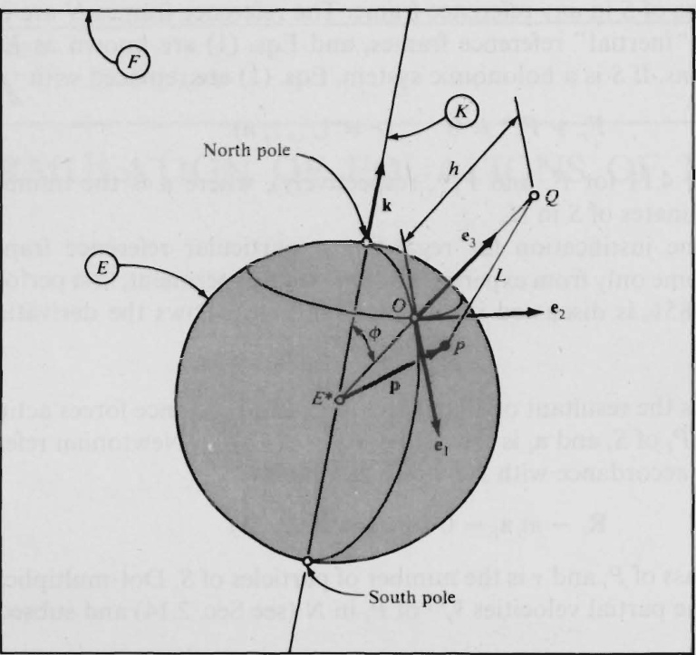
Figure 6.1.1

With a view to writing the dynamical equations governing all motions of P ,we introducegeneralized speeds u_{1} and u_{2} as

u_{\bar{r}}\triangleq^{E}\mathbf{v}^{P}\cdot\mathbf{b}_{r}\qquad(r=1,2)

where \varepsilon_{\mathbf{\tilde{v}}}r is thevelocityof P in E ,and {\bf b}_{1} and {\bf b}_{2} areunitvectorsdirected as shown in Fig. 6.1.3. Next, we begin the task of formulating expressions for partialvelocitiesof P in \boldsymbol{{F}} by writing

\begin{array}{r}{\mathbf{\boldsymbol{F}}_{\mathbf{V}}P\quad=\quad F_{\mathbf{V}}\boldsymbol{\bar{E}}\,+\,\varepsilon_{\mathbf{V}}P}\\ {(2.8.1)\quad}\end{array}

where E denotes that point of E with which P coincides, so that, if \pmb{\mathrm{p}} is the positionvector from E^{*} to P ,as shown in Fig. 6.1.1,

\begin{array}{r}{F_{\mathbf{V}}\widecheck E\qquad=\;\;F_{\mathbf{V}}E^{*}\;+\;{^F\mathbf{\omega}^{E}}\widecheck\mathbf{\omega}\times\mathbf{p}}\\ {(2.7.1)\qquad\qquad\qquad\qquad\qquad\quad}\end{array}

or, since

F_{\mathbf{V}}{}^{E^{*}}=0

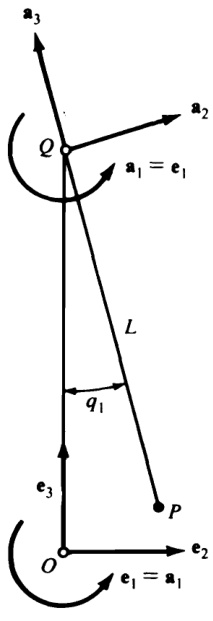
Figure 6.1.2

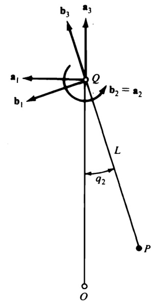
Figure 6.1.3

then, by hypothesis, we have

{}^{F}\mathbf{v}^{\bar{E}}\ =\ {}^{F}\mathbf{\Theta}\mathbf{\Theta}^{E}\times\ \mathbf{p}=\omega\mathbf{k}\ \times\ \mathbf{p}

Asfor \pmb{{\cal E}}_{\mathbf{v}}\pmb{{\cal P}} it follows directly from Eqs. (6) together with the fact that \varepsilon_{\mathbf{v}}P\cdot{\mathbf{b}}_{3}=0 (because \pmb{{\cal E}}_{\mathbf{v}}\pmb{{\cal P}} must be perpendicular to {\bf b}_{3}. ) that (see Sec. 1.3)

\varepsilon_{\mathbf{v}}P=u_{1}\mathbf{b}_{1}+u_{2}\mathbf{b}_{2}

Thus,

{\mathbf{\Sigma}}^{F}{\mathbf{v}}^{P}=\omega{\mathbf{k}}{\mathbf{\Sigma}}{\times}{\mathbf{\Sigma}}{\mathbf{p}}+u_{1}{\mathbf{b}}_{1}+u_{2}{\mathbf{b}}_{2}

and the partial velocities of P in F are simply

^{F}\mathbf{v_{1}}^{P}\:=\:\mathbf{b}_{1}\qquad^{F}\mathbf{v_{2}}^{P}\:=\:\mathbf{b}_{2}

The acceleration of P in F , required in connection with the generalized inertia forces for \pmb{P} in {\pmb F} , is given by

{}^{F}{\bf a}^{P}\;\;=\;\;{}^{F}{\bf a}^{\bar{E}}+{}^{E}\!\!\hat{{\bf a}}^{P}+2^{F}{\bf\omega}^{E}\times{}^{E}{\bf v}^{P}

with

\begin{array}{r l}{\ {^F_{\mathbf{a}}}\bar{^E}}&{\!=\!\begin{array}{c}{{^F{\mathbf{a}}}{^{E^{*}}}+{^{\ F}\!\mathbf{\Sigma}_{0}}{^{E}}\times{^{(F}\!\mathbf{\Sigma}_{0}^{E}}\times\mathbf{\Sigma}\mathbf{\Sigma})+{^{F}\!\mathbf{\Sigma}_{\alpha}}{^{E}}\times\mathbf{p}}\\ {(2.7.2)}\end{array}}\\ &{\!=\!\begin{array}{c}{{0+\omega^{2}\mathbf{k}\times(\mathbf{k}\times\mathbf{p})+0}}\\ {(5)}\end{array}}\\ {\ {^E_{\mathbf{a}}}{^{P}}}&{\!=\!\begin{array}{c}{{^E\!\mathbf{d}}}\\ {(2.6.2)\overline{{d t}}\!\left({^{E}\!\mathbf{v}}^{P}\right)\!\!\!}&{\!\!\!=\!\!\!\!}&{\!\!\!i_{1}\mathbf{b}_{1}+\dot{u}_{2}\mathbf{b}_{2}}\end{array}

and

2^{F}\pmb{\upomega}^{E}\,\times\,^{E}\!\mathbf{v}^{P}=2\omega\mathbf{k}\,\times\,(u_{1}\mathbf{b}_{1}\,+\,u_{2}\,\mathbf{b}_{2})

so that

{}^{F}\!{\bf a}^{P}\,=\,\omega^{2}\!\mathrm{\bf~k}\,\times\,({\bf k}\,\times\,{\bf p})\,+\,\dot{u}_{1}{\bf b}_{1}\,+\,\dot{u}_{2}\,{\bf b}_{2}\,+\,2\omega\mathrm{\bf~k}\,\times\,(u_{1}{\bf b}_{1}\,+\,u_{2}\,{\bf b}_{2})

Hence, the generalized inertia forces for \pmb{P} in F ,given by

F_{r}^{{\bf\Pi}_{*}}\quad=\quad_{^{F}\!{\bf v}_{r}^{~P}}\!\cdot(-m^{F}{\bf a}^{P})\qquad(r=1,2)

where m is the mass of P ,are

and

\begin{array}{r}{F_{1}\mathbf{\Pi}_{(19,13,18)}^{*}=\quad\quad-m[\omega^{2}\mathbf{k}\times(\mathbf{k}\times\mathbf{p})\mathbf{\cdotb}_{1}+\Dot{u}_{1}-2\omega u_{2}\mathbf{k}\cdot\mathbf{b}_{3}]}\\ {\quad}\\ {F_{2}\mathbf{\Pi}_{(19,13,18)}^{*}-m[\omega^{2}\mathbf{k}\times(\mathbf{k}\times\mathbf{p})\mathbf{\cdotb}_{2}+\Dot{u}_{2}+2\omega u_{1}\mathbf{k}\cdot\mathbf{b}_{3}]}\end{array}

The only contact force acting on P is the force exerted on P by the string connecting \pmb{P} to Q . Since the string is presumed to be “light,”" the line of action of this force is regarded as parallel to {\bf b}_{3} , and the force contributes nothing to the generalized active forces F_{1} and F_{2} for \boldsymbol{s} in \pmb{F} because the partial velocities \bar{F}_{\mathbf{v}_{1}}\bar{P} and {\cal F}_{{\bf v}_{2}}{}^{P} [see Eqs. (13)] are perpendicular to {\bf b}_{3} . By way of contrast, the gravitational force \mathbf{G} exerted on \pmb{P} by {\pmb E} given by

\mathbf{G}_{_{(4.8.1)}}-m g\mathbf{e}_{3}

where \pmb{g} is the gravitational acceleration at o , does contribute to \boldsymbol{F}_{1} and F_{2} Hence,

F_{r}=\mathbf{G}\cdot^{F}\mathbf{v}_{r}^{\;\;P}\;=\;-m g\mathbf{e}_{3}\cdot^{F}\mathbf{v}_{r}^{\;\;P}\;\;\;\;\;\;\;(r=1,2)

so that

F_{1}\,=\,-\,m g\mathbf{e}_{3}\cdot\mathbf{b}_{1}\qquad F_{2}\,=\,-\,m g\mathbf{e}_{3}\cdot\mathbf{b}_{2}

and substitution from Eqs. (24), (20), and (21) into Eqs. (2) yields

\begin{array}{c}{{\dot{u}_{1}=-\omega^{2}\mathbf{k}\times(\mathbf{k}\times\mathbf{p})\cdot\mathbf{b}_{1}+2\omega u_{2}\,\mathbf{k}\cdot\mathbf{b}_{3}-g\mathbf{e}_{3}\cdot\mathbf{b}_{1}}}\\ {{\dot{u}_{2}=-\omega^{2}\mathbf{k}\times(\mathbf{k}\times\mathbf{p})\cdot\mathbf{b}_{2}-2\omega u_{1}\mathbf{k}\cdot\mathbf{b}_{3}-g\mathbf{e}_{3}\cdot\mathbf{b}_{2}}}\end{array}

The leading term in each of these equations may be dropped because it is approximately four orders of magnitude smaller than the last term in each equation. As for the dot products \mathbf{e}_{3}\cdot\mathbf{b}_{1} and \mathbf{e}_{3}\cdot\mathbf{b}_{2} , reference to Figs. 6.1.2 and 6.1.3 permits one to express these as

\mathbf{e}_{3}\cdot\mathbf{b}_{1}=\,-\mathbf{c}_{1}\mathbf{s}_{2}\qquad\mathbf{e}_{3}\cdot\mathbf{b}_{2}=\mathbf{s}_{1}

and, if \phi is the angle between line K and line F^{*}O (see Fig. 6.1.1), then {\bf k}\cdot{\bf b}_{3} is given by

\mathbf{k}\cdot\mathbf{b}_{3}=\mathsf{c}_{1}\mathsf{c}_{2}\mathsf{c}\phi-\mathsf{s}_{2}\mathsf{s}\phi

Hence, if F is a Newtonian reference frame, the dynamical equations governing all motions of P are

\begin{array}{r}{\dot{u}_{1}\ =\ 2\omega u_{2}(\mathtt{c}_{1}\mathtt{c}_{2}\mathtt{c}\phi\ -\ \mathtt{s}_{2}\mathtt{s}\phi)+g\mathtt{c}_{1}\mathtt{s}_{2}}\\ {\mathrm{(25)}\qquad\qquad\qquad\qquad\mathtt{(28)}}\\ {\dot{u}_{2}\ =\ -2\omega u_{1}(\mathtt{c}_{1}\mathtt{c}_{2}\mathtt{c}\phi-\mathtt{s}_{2}\mathtt{s}\phi)-g\mathtt{s}_{1}}\\ {\qquad\qquad\qquad\qquad\qquad\mathtt{(28)}}\end{array}

Since Eqs. (29) and (30) involve four unknown functions of time, namely, u_{1},\,u_{2},\,q_{1}. and q_{2} ,.they must be supplemented by two additional equations before they can be used to produce motion predictions. The required additional equations are kinematical relationships obtained by taking advantage of the fact that E_{\mathbf{v}}P is given not only by Eq. (11), but also by (see Fig. 6.1.3)

\varepsilon_{\mathbf{v}^{P}}\underset{(2.6,1)}{=}\frac{\varepsilon_{d}}{d t}(-L\mathbf{b}_{3})\underset{(2.1,2)}{=}-L^{E}\mathbf{\upomega}^{B}\times\,\mathbf{b}_{3}

where \pmb{{\cal E}}_{\mathbf{0}}\mathbf{\mathrm{p}}^{B} is the angular velocity in E of a reference frame \textbf{\emph{B}} in which \ensuremath{\mathbf{b}}_{1},\,\ensuremath{\mathbf{b}}_{2} ， and {\bf b}_{3} are fxed ; that is (see Figs. 6.1.2 and 6.1.3),

{\dot{\bf{\sigma}}}{\bf{\sigma}}^{B}={\dot{q}}_{1}{\bf{a}}_{1}+{\dot{q}}_{2}{\bf{b}}_{2}={\dot{q}}_{1}({\bf{c}}_{2}{\bf{b}}_{1}+{\bf{s}}_{2}{\bf{b}}_{3})+{\dot{q}}_{2}{\bf{b}}_{2}

Consequently,

\begin{array}{r}{\boldsymbol{\varepsilon}_{\mathbf{v}}\mathbf{\rho}_{\parallel}^{P}=\quad-L(\dot{q}_{2}\mathbf{b}_{1}-\dot{q}_{1}\mathbf{c}_{2}\mathbf{b}_{2})}\end{array}

and, comparing this equation with Eq. (11), one concludes that the needed equationsare

\dot{q}_{1}=\frac{u_{2}}{L\mathsf{c}_{2}}\qquad\dot{q}_{2}=\,-\frac{u_{1}}{L}

Since Eqs. (29), (30), and (34) form a set of coupled, nonlinear differential equations, they cannot be solved in closed form. However, particular solutions, corresponding to specific initial conditions, can be obtained by solving the equations numerically (a subject discussed in its own right in Sec. 7.5). Suppose, for instance, that L=10\textrm{m} \phi=45^{\circ} and q_{1},\,q_{2},\,u_{1},\,u_{2} have the following initial values:

q_{1}(0)=10^{\circ}\qquad q_{2}(0)=u_{1}(0)=u_{2}(0)=0

In other words, P is initially displaced toward the east in such a way that the string makes an angle of 10^{\circ} with the local vertical, and \pmb{P} is then released from a state of rest in E [see Eqs. (11) and (35)]. The numerical solution of Eqs. (29), (30), and (34) corresponding to these initial conditions (and \omega=7.29\,\times 10^{-\,5}~\mathrm{{rad/s}} g=9.81\ \mathrm{m}/\mathrm{s}^{2}) leads to q_{1} and \boldsymbol{q}_{2} values such as those recorded in columns 2 and 3 of Table 6.1.1. Columns 4 and 5 show the values one obtains when one assumes that E rather than {\pmb F} is a Newtonian reference frame, results that can be generated by using Eqs.(29) and (30) with \omega=0. The two sets of results can be seen to agree with each other rather well as regards q_{1} but differ from each other markedly as regards \boldsymbol{q}_{2} . To determine whether column 3 or column 5 corresponds more nearly to reality, it is helpful to proceed as follows.

Table 6.1.1

<html>

	Fregarded asNewtonian		EregardedasNewtonian
1 t(s)	2 q1 (deg)	3 q2 (deg)	4 q1 (deg)	5 q2 (deg)
0.0 2.0	10.00000 ~3.95462	0.00000 0.00088	10.00000 -3.95462	0.00000 0.00000
4.0	-6.87785	0.00105	-6.87785	0.00000
6.0	9.38832	-0.00306	9.38832	0.00000
8.0	-0.54571	0.00068	-0.54571	0.00000
10.0	-8.95764	0.00442	-- 8.95764	0.00000
12.0	7.62749	-0.00496	7.62749	0.00000
14.0	2.93028	-0.00180	2.93028	0.00000
16.0	-9.94059	0.00815	-9.94059	0.00000
18.0	4.93175	-0.00475	4.93176	0.00000
20.0	6.04627	-0.00612	6.04628	0.00000
22.0	9.70738	0.01100	-9.70739	0.00000
24.0	1.63058	-0.00198	1.63058	0.00000
26.0	8.42042	-0.01134	8.42042	0.00000
28.0	-8.28631	0.01180	-8.28632	0.00000
30.0	-1.87098	0.00324	-1.87098	0.00000
32.0	9.76306	-0.01617	9.76307	0.00000
34.0	-5.85006	0.00975	-5.85006	0.00000
36.0	-5.14262	0.01016	-5.14263	0.00000
38.0	9.91107	-0.01925	9.91109	0.00000
40.0	2.69598	0.00456	-2.69599	0.00000
42.0	-7.78299	0.01757	-7.78301	0.00000
44.0	8.84651	-0.01939	8.84653	0.00000
46.0	0.78933	-0.00340	0.78934	0.00000
48.0	-9.46949	0.02393	-9.46952	0.00000
50.0	6.69863	-0.01583	6.69865	0.00000
52.0	4.17764	-0.01310	4.17766	0.00000
54.0	-9.99698	0.02771	9.99702	0.00000
56.0	3.72919	-0.00841	3.72920	0.00000
58.0	7.05291	-0.02300	7.05295	0.00000
60.0	9.30148	0.02762	-9.30152	0.00000

</html>

Let r be the position vector from o to P^{*} , the orthogonal projection of P on the horizontal plane passing through o , as shown in Fig. 6.1.4. Then

\mathbf{r}=L\mathbf{e}_{3}\times(\mathbf{e}_{3}\times\mathbf{b}_{3})

or, since \mathbf{b}_{3}=\mathbf{s}_{2}\mathbf{e}_{1}\,-\,\mathbf{s}_{1}\mathbf{c}_{2}\mathbf{e}_{2}\,+\,\mathbf{c}_{1}\mathbf{c}_{2}\mathbf{e}_{3},

\mathbf{r}=L(-\mathbf{s}_{2}\mathbf{e}_{1}+\mathbf{s}_{1}\mathbf{c}_{2}\mathbf{e}_{2})

Hence, if E_{1} and E_{2} are Cartesian coordinate axes passing through o and parallel to \mathbf{e}_{1} and \mathbf{e}_{2} ，respectively, then the E_{1} and E_{2} coordinates of P^{*} are -L s_{2} and L s_{1}\mathbf{c}_{2} , respectively, and one can plot the path traced out by P^{\ast} in the E_{1}{\mathrm{-}}E_{2} plane, as has been done in Fig. 6.1.5 with data corresponding to columns 2 and 3 of Table 6.1.1; a portion of the E_{2} axis represents columns 4 and 5 since, with q_{2}=0 , Eq. (37) reduces to

{\bf r}=L s_{1}{\bf e}_{2}

Figure 6.1.5 shows that the assumption that F is a Newtonian reference frame leads to the prediction that P^{*} must trace out a complicated curve in the E_{1}{\mathrm{-}}E_{2} plane. If it is assumed that E is a Newtonian reference frame, then the path predicted for P^{*} is simply a straight line. Foucault's experiments, performed at the Pantheon in Paris and subsequently duplicated in numerous other locations, revealed that P^{*} moves on a curve such as the one in Fig. 6.1.5. Moreover, good quantitative agreement was obtained between experimental data and values predicted mathematically. Hence, regarding F as a Newtonian reference frame is more realistic than assuming that E is a Newtonian reference frame. But this does not mean that F is, in fact, a Newtonian reference frame or that one may not regard E as such a reference frame in certain contexts.

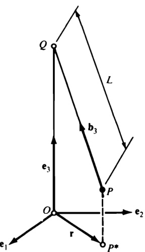
Figure 6.1.4

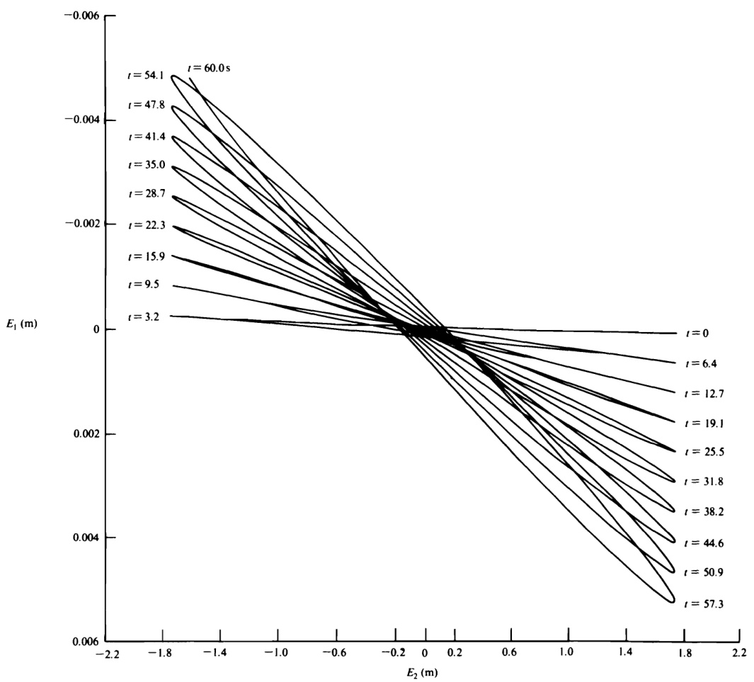
Figure 6.1.5

6.2 SECONDARY NEWTONIAN REFERENCE FRAMES

Astronomical observations furnish a large body of data showing that the reference frame F of the example in Sec. 6.1 is not a Newtonian reference frame, because motion predictions based on Eqs. (6.1.1) or (6.1.2) together with the assumption that F is such a reference frame conflict with the data. This fact suggests the following question: Why does the hypothesis that F is a Newtonian reference frame lead to a satisfactory description of the motion of a pendulum relative to the Earth, but to an incorrect description of, for example, the motion of the. Moon relative to the Earth? This question and a number of related ones can be answered in the light of the following theorem:

If N^{\prime} is a reference frame performing a prescribed motion relative to a Newtonian reference frame N ,then N^{\prime} is a Newtonian reference frame throughout some time interval if and only if throughout this time interval the acceleration in N of every point of N^{\prime} is equal to zero. When a reference frame moves in such a way that the acceleration of each of its points in a Newtonian reference frame is equal to zero, it is called a secondary Newtonian reference frame.

Proof If P is any particle of a system S, then the partial velocities of P in N and in N^{\prime} are equal to each other since the velocities of P in N and in N^{\prime} differ from each other only due to the motion of N^{\prime} relative to N , which, being prescribed, does not involve the generalized speeds for s in N , and hence does not affect the partial velocities. Consequently, the generalized active force {\widetilde{\boldsymbol{F}}}, for s in N is necessarily equal to the generalized active force \widetilde{F}_{r}^{\,\prime}\left(r=1,\ldots,p\right) for s in N^{\prime} , no matter how N^{\prime} moves in N ; but the generalized inertia force \widetilde{F}_{r}{}^{*} for s in N can differ from the generalized inertia force \widetilde{F}_{r}{}^{*\prime} for s in N^{\prime} due to differences in the accelerations NaP and NaP. Now,

^N\mathbf{a}^{P}\underset{(2.8.1)}{=}^{N^{\prime}}{\mathbf{a}^{P}}+\,^{N}\!\mathbf{a}^{\bar{N}^{\prime}}+2^{N}\!\mathbf{\omega}^{N^{\prime}}\times\,^{N^{\prime}}\mathbf{v}^{P}

where \overline{{N}}^{\prime} is the point of N^{\prime} that coincides with \pmb{P} . Furthermore, if ^o is any point fixed in N^{\prime} , then

\begin{array}{r l r}{^N\mathbf{\underline{{a}}}^{N^{\prime}}}&{=}&{^N\mathbf{\underline{{a}}}^{O}+^{N}\!\!\!\alpha^{N^{\prime}}\times\mathbf{r}+^{N}\!\!\!\mathfrak{w}^{N^{\prime}}\times(^{N}\!\!\!\mathfrak{w}^{N^{\prime}}\times\mathbf{r})}\end{array}

where r is the position vector from o to \bar{N}^{\prime} . Hence, if the acceleration in N of every point of N^{\prime} is equal to zero, so that

^N\mathbf{\mathfrak{a}}^{\vec{N}^{\prime}}={}^{N}\mathbf{\mathfrak{a}}^{o}=0

then

^N\!\!\!\mathfrak{a}^{N^{\prime}}\,\times\,\mathbf{r}\,+\,^{N}\!\!\mathfrak{a}^{N^{\prime}}\,\times\,(^{N}\!\!\mathfrak{a}^{N^{\prime}}\,\times\,\mathbf{r})\ =\ 0

and this can be satisfied for all r only if

N_{\pmb{\alpha}^{N^{\prime}}}=0

and

^N{\bf\epsilon}_{\bf G}^{N^{\prime}}=0

in which event

\begin{array}{r l r}{N_{\mathbf{a}}P}&{{}=}&{N_{\mathbf{\a}}P}\end{array}

and, therefore [see Eqs. (4.11.1) and (4.11.3)],

\tilde{F}_{r}{^*}=\tilde{F}_{r}{^*}\qquad(r=1,\ldots,p)

which means that whenever \tilde{F}_{r}+\tilde{F}_{r}{}^{*}=0\ \left(r=1,\ldots,p\right)\, then \widetilde{F}_{r}^{\;\prime}+\widetilde{F}_{r}{}^{*\prime}=0 (r=1,\ldots,p) and, consequently, that N^{\prime} is a Newtonian reference frame.

To show that N^{\prime} is not a Newtonian reference frame unless the acceleration in N of every point of N^{\prime} is equal to zero, let o be a point of N^{\prime} such that

\mathbf{v_{z}}o\neq0

and let Sconsist of a single particle P situatedpermanently at o .Then

\mathbf{v^{\prime}}_{\mathbf{a}}P=0

while

^N\mathbf{a}^{P}\ =\ \ 0\ +\ ^{N}\mathbf{a}^{O}+\ \ 0\ \neq0

so that

\begin{array}{c c}{{}^{N}{\bf a}^{P}}\end{array}\nrightarrow\begin{array}{c}{{\nrightarrow}}\\ {{(10,11)}}\end{array}

and, therefore,

\tilde{F}_{r}{^*}\ne\tilde{F}_{r}{^*}\,\qquad(r=1,\dots,p)

which means that whenever \tilde{F}_{r}+\tilde{F}_{r}{}^{*}=0\ \ (r=1,\ldots,p), then \widetilde{F}_{r}^{\;\prime}\,+\,\widetilde{F}_{r}{}^{*\prime}\ne0 (r=1,\hdots,p) and, consequently,that N^{\prime} is not a Newtonian reference frame.

Returning to the question raised at the beginning of the section, we let A be a reference frame in which the Sun s remains fixed and relative to which the orientation of thereference frame F introduced in the example in Sec. 6.1 does not vary, so that {}^{A}{\bf60}^{F}=0 , but in which the center E^{*} of the Earth E moves on a plane curve. A,S,F ,and E are depicted in Fig. 6.2.1, which also shows the Moon M

Suppose that A is a Newtonian reference frame.Then F cannot possibly be a Newtonian reference frame, because there exists no point of F whose acceleration in A is equal to zero. In fact, the acceleration in A of every point that is fixed in F is equal to the acceleration {\bf\Psi_{a}}^{E^{*}} of E^{*} in A , and this acceleration has a magnitude that can be estimated with suffcient accuracy for present purposes by assuming that E^{*} moves in A on a circle of radius R\approx1.5\,\times\,10^{11}\,\mathrm{m} traced out once per year. How important is this acceleration? That depends on the acceleration in F of the particles of the system under consideration.As the angular velocity of F in A is equal to zero, and,hence, the angular acceleration of F in A is also equal to zero, the acceleration A_{\mathbf{a}}P of a particle P in A differs from the acceleration F_{\mathbf{a}}P of P in F by precisely \mathbf{\Psi_{a}}^{E^{*}} . Errors resulting from regarding F , rather than A as a Newtonian reference frame therefore grow in importance as the ratio of |\,^{A}\mathbf{a}^{E^{\ast}}| to |^{F}\mathbf{a}^{P}| increases. Hence, in connection with studies of motions of the Moon, an object whose particles move in {\pmb F} , essentially, on circles having radi of approximately 4.0\,\times\,10^{8}\,\mathrm{m}, . each particle completing about 12 such orbits per year, it must make a substantial difference whether \pmb{A} or F is assigned the role of Newtonian reference frame, because the ratio in question here has the value (let \pmb{F}_{\mathbf{\mathbf{g}}}\pmb{M} be the acceleration in {\pmb F} of a typical particle of the Moon)

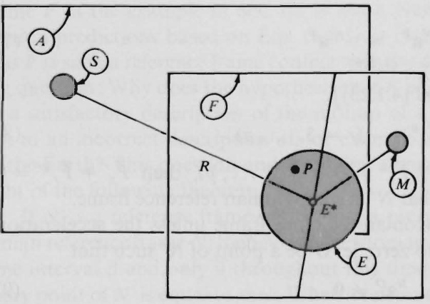
Figure 6.2.1

\frac{|^{A}\mathbf{a}^{E^{*}}|}{|^{F}\mathbf{a}^{M}|}=\frac{1.5\,\times\,10^{11}}{4.0\,\times\,10^{8}}\left(\frac{1}{12}\right)^{2}\approx2.6

which means that |\,^{A}\mathbf{a}^{E*}| cannot be regarded as negligible in comparison with |\pmb{F_{\mathbf{a}}^{M}}| By way of contrast, for the pendulum considered in Sec. 6.1, \pmb{g}\pmb{\alpha} is a reasonable upper bound for $|{}^{F}\mathbf{a}^{P}|.$ where \pmb{\alpha} is the maximum value of the angle between lines o Q and P Q in Fig. 6.1.1, so that, with g=9.81\;\mathrm{m}/\mathrm{s}^{2} and \pmb{\alpha} even as small as 0.01 rad,

\frac{|^{A}\mathbf{a}^{E^{*}}|}{|^{F}\mathbf{a}^{P}|}\approx0.06

Thus, so far as numerical results are concerned, it here matters far less whether \pmb{A} or F is regarded as a Newtonian reference frame.

As was pointed out in Sec. 6.1, the pendulum experiments performed by Foucault support the hypothesis that {\pmb F} is a Newtonian reference frame. Now [see Eq. (15)] we see that these experiments support the same hypothesis for \pmb{A} ， but that comparisons of actual with predicted motions of the Moon can reveal which of these two reference frames is the stronger contender for the title of " true” Newtonian reference frame. It turns out that \pmb{A} is the winner of this contest. But this is not to say either that A actually is a Newtonian reference frame or that Eqs. (6.1.1) or (6.1.2) should be used only in conjunction with \pmb{A} (rather than with F Phenomena such as the nutation of the Earth and the motion of the Sun relative to the galaxy as a whole show that \pmb{A} falls short of perfection. Moreover, the use of \pmb{A} in place of F is desirable only when it makes a discernible difference; otherwise it merely complicates matters. Similarly, treating the Earth, rather than \pmb{A} or F as a Newtonian reference frame is sound practice whenever doing so leads to analytical simplifications unaccompanied by significant losses in accuracy, as is the case in a large number of situations encountered in engineering. Hence, unless explicitly exempted, every use of Eqs. (6.1.1) or (6.1.2) in the remainder of this book will be predicated on the assumption that allreference frames rigidly attached to the Earth, as well as all reference frames all of whose points have zero acceleration relative to the Earth, may be regarded as Newtonian reference frames.

6.3 ADDITIONAL DYNAMICAL EQUATIONS

When generalized speeds are introduced in addition to u_{1},\dotsc,u_{p} for the purpose of bringing into evidence forces and/or torques that contribute nothing to the generalized active forces \widetilde{F}_{1},...,\widetilde{F}_{p} or, if s is a holonomic system, to F_{1},\ldots,F_{n} ， then the dynamical equations corresponding to the additional generalized speeds furnish the needed information about the forces and/or torques in question. To generate these dynamical equations, follow the procedures set forth in Secs. 4.9 and 4.11 to form expressions for the generalized active forces and generalized inertia forces corresponding to the additional generalized speeds, and then substitute into Eqs. (6.1.1) or (6.1.2).

Example When the bearing surface \pmb{B} and the rod \pmb R of the system introduced in the example in Sec. 4.9 and depicted in Fig. 4.9.1 both are perfectly smooth, the dynamical equations governing the motion of the system, written by substituting from Eqs. (4.9.6), (4.9.7), (4.11.35), and (4.11.36) into Eqs. (6.1.1), are

\begin{array}{l}{{\dot{u}_{1}=g\cos\beta+q_{1}(u_{2}\sin\beta)^{2}}}\\ {{\dot{u}_{2}=\cfrac{T\csc^{2}\beta-2m q_{1}u_{1}u_{2}}{{m\pmb q_{1}}^{2}+4M L^{2}/3}}}\end{array}

and these, together with the kinematical equation

\dot{q}_{1}\mathop{=}_{(4.9.2)}u_{1}

permit one to determine \mathbf{\mathit{q}_{1}},\,\mathbf{\mathit{u}_{1}} , and \pmb{u}_{2} for t>0 when the values of these variables are known for t=0 (and _{T} has been specified as a function of \pmb q_{1} u_{1},\,u_{2} , and t ). But if, as in the example in Sec. 4.10, the contact between the sleeve s and the bearing surface B_{\mathrm{{c}}} as well as the contact between \pmb{P} and \pmb R is presumed to take place across a rough surface, then Eqs. (4.10.39) and (4.10.40) replace Eqs. (4.9.6) and (4.9.7), respectively, with the result that the dynamical equations become

\dot{u}_{1}=g\cos\beta-\bigg(\frac{\mu_{1}^{\prime}}{m}\bigg)({\rho_{2}}^{2}+\rho_{3}^{2})^{1/2}\,\mathrm{sgn}\,u_{1}+q_{1}\,(u_{2}\,\sin\beta)^{2}

{\dot{u}}_{2}={\frac{\left[T\,-\,(2\pi n^{*}/3)({b_{2}}^{3}-{b_{1}}^{3}){\mu_{2}}^{\prime}\ {\mathrm{sgn}}\,u_{2}\right]\,{\mathrm{csc}}^{2}\,\beta\,-\,2m q_{1}u_{1}u_{2}}{{m q_{1}}^{2}+4{M L}^{2}/3}}

and, since these contain \rho_{2},\,\rho_{3} , and n^{\ast} , they do not suffice [together with Eq. (3)] for the determination of q_{1},u_{1} , and \pmb{u}_{2} . However, one can supplement Eqs. (3)-(5) with the dynamical equations corresponding to u_{3},\,u_{5} , and \pmb{u_{9}} as introduced in Sec. 4.9 [see Eqs. (4.9.11), (4.9.15), and (4.9.24), respectively]. These equations are

\begin{array}{r}{(m+M)g-\pi{n^{*}({b_{2}}^{2}-{b_{1}}^{2})}-m\dot{u}_{1}\cos\beta\underset{(4.11.37)}{=}0}\\ {\rho_{3}\mathrm{~\qquad~}-m(\dot{u}_{2}q_{1}+2u_{1}u_{2})\sin\beta\underset{(6.11.39)}{=}0}\end{array}

and with their aid one can eliminate n^{*} ， \rho_{2} , and \rho_{3} from Eqs. (4) and (5) and thus come into position to determine \boldsymbol{q}_{1},\boldsymbol{u}_{1} , and u_{2} as functions of t

6.4 LINEARIZATION OF DYNAMICAL EQUATIONS

Frequently, one can obtain much useful information about the behavior of a system s from linearized forms of kinematical and/or dynamical equations, that is, equations derived from nonlinear equations by omitting all terms of second or higher degree in perturbations of some (or all) of the generalized speeds u_{1},\ldots,u_{n} and generalized coordinates q_{1},\ldots;q_{n} . This is true primarily because linear differential equations generally can be solved more easily than can nonlinear differential equations. Of course, the solutions of such linearized equations lead one only to approximations of the solutions of the corresponding full, nonlinear equations; and they may be rather poor approximations. In any event, however, the approximations become ever better as the perturbations involved in the linearization take on ever smaller values.

When nonlinear kinematical and/or dynamical equations are in hand, one forms their linearized counterparts by expanding all functions of the perturbations involved in the linearization into power series in these perturbations and dropping all nonlinear terms. To formulate linearized dynamical equations directly, that is, without first writing exact dynamical equations, proceed as follows:

Develop fully nonlinear expressions for angular velocities of rigid bodies belonging to S, for velocities of mass centers of such bodies, and for velocities of particles of s to which contact and/or distance forces contributing to generalized active forces are applied. Use these nonlinear expressions to determine partial angular velocities and partial velocities by inspection. Linearize all angular velocities of rigid bodies and velocities of particles, and use the linearized forms to construct linearized angular accelerations and accelerations. Linearize all partial angular velocities and partial velocities. Form linearized generalized active forces and linearized generalized inertia forces, and substitute into Eqs. (6.1.1) or (6.1.2).

Examples As was shown in the example in Sec. 6.1, all motions of the Foucault pendulum are governed by the equations

\begin{array}{r l}&{\dot{u}_{1\,\,\,\,\,=\,\,\,\,2\omega u_{2}}(\mathtt{c}_{1}\mathtt{c}_{2}\mathtt{c}\phi\,-\,\mathtt{s}_{2}\,\mathtt{s}\phi)+g\mathtt{c}_{1}\mathtt{s}_{2}}\\ &{\qquad\overset{(6.1.29)}{\underbrace{(6.1.29)}}-2\omega u_{1}(\mathtt{c}_{1}\mathtt{c}_{2}\mathtt{c}\phi-\mathtt{s}_{2}\,\mathtt{s}\phi)-g\mathtt{s}_{1}}\end{array}

\dot{q}_{1}\mathop{=}_{(6.1.34)}\frac{u_{2}}{L\mathrm{c}_{2}}\qquad\dot{q}_{2}\mathop{=}_{(6.1.34)}-\frac{u_{1}}{L}

As may be verified by inspection, these equations possess the solution

u_{1}=u_{2}=q_{1}=q_{2}=0\qquad\quad.

Hence, one may hope to obtain useful information regarding the motion of the pendulum by employing equations resulting from linearization of Eqs. (1)-(3) “about this solution,” that is, by replacing u_{1},u_{2},q_{1} and q_{2} with perturbation functions {u_{1}}^{*},\,{u_{2}}^{*},\,{q_{1}}^{*}, and {q_{2}}^{*} , respectively, and then linearizing in these perturbations. For example, when {{u}_{1}}^{*} and {{u}_{2}}^{*} are written in place of u_{1} and \pmb{u}_{2} , respectively, in Eq. (1), and \mathbf{c}_{1},\mathbf{c}_{2} , and {\bf s}_{2} are replaced with 1, 1, and {q_{2}}^{*} , respectively, these being the terms of degree less than 2 in the expansions of cos {q_{1}}^{*} ,cos {q_{2}}^{*} , and sin {q_{2}}^{*} , respectively, then \dot{u}_{1}{}^{\ast} is given by

\dot{u}_{1}{}^{*}=2\omega u_{2}{}^{*}(\mathrm{c}\phi-q_{2}{}^{*}\mathrm{s}\phi)+g q_{2}{}^{*}

This, however, is an incompletely linearized equation because. {u_{2}}^{*}{q_{2}}^{*} isa second-degree term. Dropping this term, one arrives at the linear equation corresponding to Eq. (1), namely,

\dot{u}_{1}{}^{*}=2\omega u_{2}{}^{*}\mathrm{c}\phi+g q_{2}{}^{*}

Similarly, the linear equations corresponding to Eqs. (2) and (3) are found to be

\dot{u}_{2}{}^{*}=\,-2\omega u_{1}{}^{*}\mathrm{c}\phi\,-\,g q_{1}{}^{*}

and

\dot{q}_{1}{^*}=\frac{{u_{2}}^{*}}{L}\qquad\dot{q}_{2}{^*}=\,-\frac{{u_{1}}^{*}}{L}

To solve Eqs. (6)-(8), and thus to obtain a detailed, approximate, analytical description of the motion of the pendulum, it is helpful to introduce \pmb{\uprho} asthe linearized form of the vector r shown in Fig. 6.1.4, that is, to let

{\bf\mathfrak{p}}_{(6.1.37)}L(-q_{2}{^{*}}{\bf e}_{1}+q_{1}{^{*}}{\bf e}_{2})

for it may be verified by carrying out the indicated differentiations that Eqs. (6)-(8) are together equivalent to the single linear vector differential equation

\frac{{}^{E}d^{2}\mathbf{p}}{d t^{2}}+2\omega c\phi\mathbf{e}_{3}\,\times{}\frac{{}^{E}d\mathbf{p}}{d t}+\frac{g}{L}\mathbf{p}=0

and this equation can be replaced with an even simpler one through the introduction of a reference frame R whose angular velocity in E is taken to be

\pmb{\varepsilon_{\pmb{\omega}}}^{R}\triangleq-\omega\pmb{c}\phi\mathbf{e}_{3}

which permits one to write

\begin{array}{c}{{\displaystyle\frac{^{E}d{\bf p}}{d t}_{(2.3.1)}=\frac{^{R}d{\bf p}}{d t}+{\bf\nabla}^{E}{\bf{\bf{o}}}^{R}\times{\bf{\nabla}}{\bf{\bf{\nabla}}}{\bf{\bf{\times}}}\ {\bf{\nabla}}{\bf{\bf{\times}}}{\bf{\nabla}}{\bf{\bf{\times}}}{\bf{\nabla}}{\bf{\bf{\times}}}}\\ {{\displaystyle\frac{^{E}d^{2}{\bf p}}{d t^{2}}_{(12)}=\begin{array}{c}{{\displaystyle\frac{^{R}d^{2}{\bf p}}{d t^{2}}-\omega\mathrm{c}\phi{\bf e}_{3}\times\frac{^{R}d{\bf p}}{d t}-\omega\mathrm{c}\phi{\bf e}_{3}\times\frac{^{R}d{\bf p}}{d t}}}\\ {{\displaystyle+\ (\omega\mathrm{c}\phi)^{2}{\bf e}_{3}\times({\bf e}_{3}\times{\bf p})}}\end{array}}}\end{array}

Substitution from Eqs. (12) and (13) into Eq. (10) yields

\frac{\kappa_{d}{}^{2}\mathfrak{p}}{d t^{2}}+\frac{g}{L}\mathfrak{p}=0

if, as in Sec. 6.1, terms involving \omega^{2} are dropped. Now, Eq. (14) possesses the general solution

\mathbf{\uprho}=\mathbf{A}\cos\,p t+\mathbf{B}\sin\,p t

whereA and \mathbf{\deltaB} are vectors fixed in reference frame \pmb R and \pmb{p} known as the circular natural frequency of the pendulum, is defined as

p=\left({\frac{g}{L}}\right)^{1/2}

The vectors A and \mathbf{B} depend on initial conditions. Specifically, denoting the initial values of \mathfrak{p} and \scriptstyle{^R_{d}}\mathfrak{p}/d t by {\mathfrak{p}}(0) and \textstyle{}^{R}d\pmb{\rho}(0)/d t , respectively, one can write

\mathbf{A}_{\displaystyle(1\,5)}\,\mathbf{\uprho}(0)\qquad\mathbf{B}_{\displaystyle(1\,5)}\,\frac{1}{p}\frac{\mathbf{\nabla}^{R}d\mathbf{p}(0)}{d t}

Suppose, for example, that P is initially displaced toward the east in such a way that the string makes an angle \pmb{\alpha} with the vertical, and that P is then released from a state of rest in \pmb{E} Correspondingly,

q_{1}(0)=\alpha\qquad q_{2}(0)=0\qquad u_{1}(0)=u_{2}(0)=0

Hence,

\mathrm{~\bf~r}(0)\mathrm{~\boldmath~\xi~}.\;=\;\mathrm{~\boldmath~\cal~L~}\!s\alpha{\bf e}_{2}(0)

so that linearization in \pmb{\upalpha} yields

{\pmb\rho}(0)=L\alpha{\pmb e}_{2}(0)

where {\mathfrak{e}}_{2}(0) denotes the value of \mathfrak{e}_{2} in \pmb R at \scriptstyle t\;=\;0 . Similarly, one can write

\begin{array}{l}{\displaystyle\frac{\boldsymbol{\kappa}_{d\Gamma(0)}}{d t}=\frac{\boldsymbol{\kappa}_{d\Gamma(0)}}{d t}+\mathbf{\nabla}^{R}\boldsymbol{\omega}^{E}(0)\,\times\,\mathbf{r}(0)}\\ {\displaystyle\quad=\,\boldsymbol{\kappa}_{\mathbf{v}}\boldsymbol{P}(0)\,+\,\boldsymbol{\omega}\boldsymbol{c}\phi\mathbf{e}_{3}(0)\,\times\,[L s\boldsymbol{\alpha}\mathbf{e}_{2}(0)]}\\ {\displaystyle\quad\qquad\qquad\qquad\qquad\qquad\qquad\qquad\quad(19)}\\ {\displaystyle\quad=\,\boldsymbol{(6.1.33,6.1,34,18)}-L\boldsymbol{\omega}\boldsymbol{c}\phi s\boldsymbol{\alpha}\mathbf{e}_{1}(0)}\end{array}

and, linearizing in \pmb{\alpha} , one has

\frac{{}^{R}d{\bf p}(0)}{d t}=-L\omega{\bf c}\phi\alpha{\bf e}_{1}(0)

Thus, \mathbf{\uprho} can be written

\begin{array}{r l}{\textsf{\textsf{p}}=\underbrace{L\alpha\mathbf{e}_{2}(0)\cos p t-L\left(\frac{\omega}{p}\right)\mathsf{c}\phi\alpha\mathbf{e}_{1}(0)\sin p t}_{(1\mathord{\uparrow},20)}}&{}\\ {\qquad=\underbrace{L\alpha\biggl[-\left(\frac{\omega}{p}\right)\mathsf{c}\phi\sin p t\mathbf{e}_{1}(0)+\cos p t\mathbf{e}_{2}(0)\biggr]}_{(1\mathord{\uparrow},2\mathord{\downarrow})}}\end{array}

According to Eq. (23), P^{*} (see Fig. 6.1.4) moves in \pmb R on an elliptical path having the proportions shown in Fig. 6.4.1, and P^{*} traverses this path once every 2\pi/p units of time. The ellipse, being fixed in \pmb R , rotates in E at a rate of \omega\mathbf{c}\phi radians per unit of time [see Eq. (11)], the rotation being clockwise as seen by an observer looking from point Q toward point ^o (see Fig. 6.1.4), provided that o is situated in the northern hemisphere. These predictions agree qualitatively with those obtained in Sec. 6.1 by using the full, nonlinear equations of motion, Eqs. (6.1.29), (6.1.30), and (6.1.34). To assess the merits of the linear theory in quantitative terms, one can compare |\boldsymbol{\mathbf{r}}| —-calculated by using Eq. (6.1.37) after integrating Eqs. (6.1.29), (6.1.30), and (6.1.34) numerically with \phi=45^{\circ} L=10\,\mathrm{m}. \omega=7.29\,\times\,10^{-\,5}\;\;\mathrm{rad/s} ， q_{1}(0)=\alpha. q_{2}(0)=u_{1}(0)=u_{2}(0)=0 —with |\pmb{\uprho}| as obtained by using Eq. (23). Plots resulting from such calculations are shown in Fig. 6.4.2 for \alpha=10^{\circ} 30^{\circ} ， and 60^{\circ} . The solid curves represent values of |\boldsymbol{\mathbf{r}}| , whereas the broken curves correspond to values of |{\pmb\uprho}| . As was to be expected, the agreement between the two curves associated with a given value of \pmb{\alpha} is best for \alpha=10^{\circ} and worst for \alpha=60^{\circ} . Of course, whether or not any given result obtained from linearized equations can be regarded as “good'" depends on the user's needs.

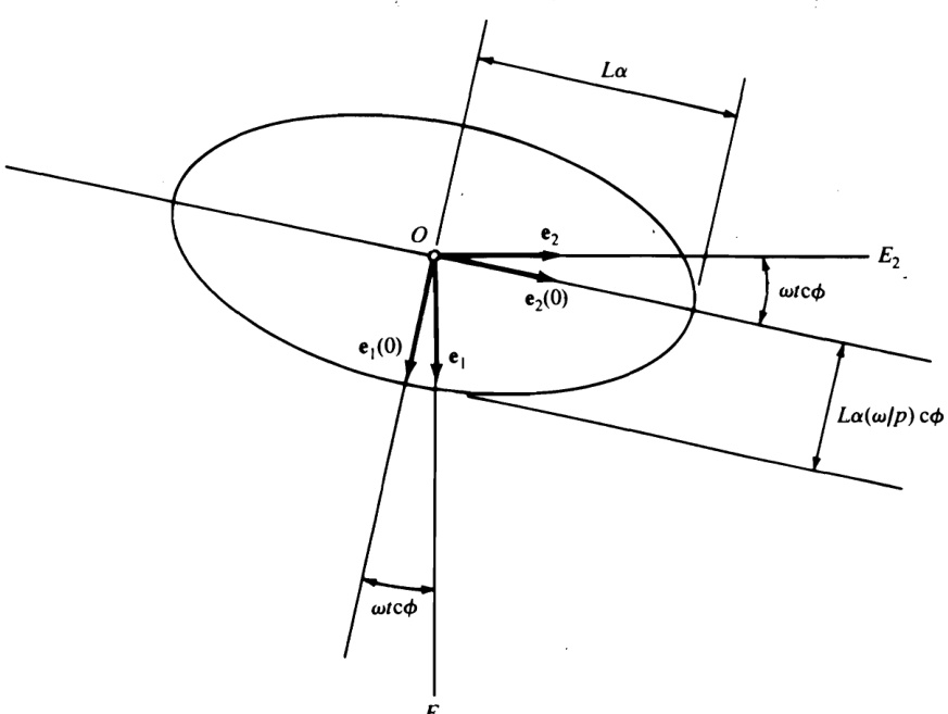
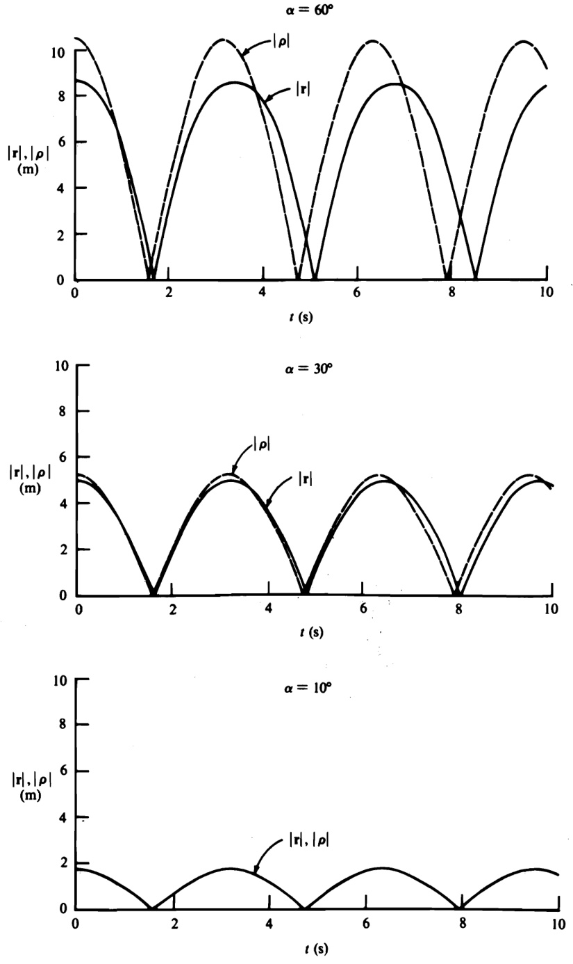
Figure 6.4.2

To illustrate the process of formulating linearized equations of motion without first constructing fully nonlinear equations, we consider a uniform bar \pmb{B} of mass m supported by frictionless sliders on a circular wire \pmb{W} of radius \pmb R , as shown in Fig. 6.4.3, and suppose that W is being made to rotate with a constant angular speed \pmb{\Omega} about a fixed vertical axis passing through the center ^o of W. Under these circumstances, it seems reasonable to suppose that \pmb{B} can remain at rest relative to W_{s} that is, that q_{1} (see Fig. 6.4.3) can have a constant value, say, \bar{\pmb q}_{1} , so that the generalized speed \pmb{u}_{1} defined as

u_{1}\triangleq\dot{q}_{1}

remains equal to zero; and one can undertake the formulation of linear equations governing perturbations {q_{1}}^{*} and {{u_{1}}^{*}} introduced by writing

q_{1}=\bar{q}_{1}+{q_{1}}^{*}\qquad u_{1}=0+{u_{1}}^{*}

One such equation is available immediately, namely,

\dot{q}_{1}{}^{*}=\,u_{1}{}^{*}

Whether or not \pmb{B} can, in fact, move as postulated, that is, whether or not there exist real values of \overline{{\boldsymbol{q}}}_{1} , will be discussed once the linearized dynamical equation governing {u_{1}}^{*} and q_{1}^{\mathrm{~*~}} has been formulated.

The angular velocity \mathbf{\delta}_{\mathbf{\delta}}^{\mathbf{\delta}} of \pmb{B} and the velocity \mathbf{v}^{\ast} of the center B^{*} of \pmb{B} are given by (see Fig. 6.4.3 for the unit vectors \ensuremath{\mathbf{b}}_{1},\ensuremath{\mathbf{b}}_{2} , and {\bf b}_{3}

\mathbf{\omega}\mathbf{\omega}=\Omega(s_{1}\mathbf{b}_{1}+c_{1}\mathbf{b}_{2})+u_{1}\mathbf{b}_{3}

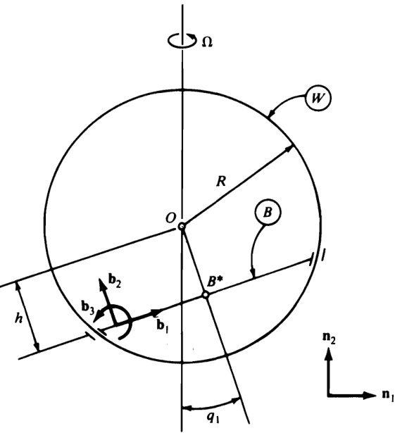
Figure 6.4.3

and

\mathbf{v}^{*}=h(u_{1}\mathbf{b}_{1}-\Omega s_{1}\mathbf{b}_{3})

respectively. Hence, the partial angular velocity {\bf{\omega}}_{1} and partial velocity {\mathbf{v}_{1}}^{*} are

\mathbf{\omega}\bullet_{1}=\mathbf{\omega}\mathbf{b}_{3}\qquad\mathbf{\nu}\mathbf{v}_{1}{}^{*}=\mathbf{\omega}h\mathbf{b}_{1}

To linearize Eqs. (27) and (28) in {q_{1}}^{*} and {{u}_{1}}^{*} ,we observe that

\mathsf{s}_{1}\,=\,\mathsf{s i n}(\bar{q}_{1}\,+\,q_{1}\,^{\ast})=\sin\bar{q}_{1}\cos q_{1}\,^{\ast}+\,\mathsf{c o s}\,\bar{q}_{1}\sin q_{1}\,^{\ast}

so that, if \bar{\bf s}_{1} and \bar{\mathsf{c}}_{1} are written in place of sin \bar{\pmb q}_{1} and cos \overline{{\boldsymbol{q}}}_{1} , respectively, and cos q_{1}^{\mathrm{~\star~}} and sin {q_{1}}^{*} are replaced with unity and {q_{1}}^{*} , respectively, then

\mathsf{s}_{1}\approx\mathsf{\bar{s}}_{1}+\mathsf{\bar{c}}_{1}q_{1}{}^{*}

Similarly,

\mathsf{c}_{1}\approx\bar{\mathsf{c}}_{1}-\bar{\mathsf{s}}_{1}q_{1}{}^{*}

Hence, the linearized forms of \mathbf{\omega} and \mathbf{v^{*}} are

{\bf{\dot{o}}}\;=\;\Omega[({\bar{s}}_{1}\,+\,{\bar{c}}_{1}{q_{1}}^{*}){\bf{b}}_{1}\,+\,({\bar{c}}_{1}\,-\,{\bar{s}}_{1}{q_{1}}^{*}){\bf{b}}_{2}]\,+\,{u_{1}}^{*}{\bf{b}}_{3}

and

\mathbf{v^{*}}\approx\left.h[u_{1}\mathbf{^{*}b}_{1}-\Omega(\bar{\mathbf{s}}_{1}+\bar{\mathbf{c}}_{1}q_{1}\mathbf{^{*}})\mathbf{b}_{3}]\right.

Asfor \mathbf{\omega}_{\mathbf{0}} and {\mathbf{v}_{1}}^{*} , these, as written in Eqs. (29), contain no terms that are nonlinear in {q_{1}}^{*} . Note, however, that {\mathbf{v}_{1}}^{*} can be written

{\mathbf{v}_{1}}^{*}\,=\,h({\mathbf{c}_{1}}{\mathbf{n}_{1}}+{\mathbf{\boldsymbol{s}}_{1}}{\mathbf{\boldsymbol{n}}_{2}})

where \mathfrak{n}_{1} and \mathbf{n}_{2} are unit vectors directed as shown in Fig. 6.4.3, and that the linearized form of {\bf v}_{1}{}^{\ast} then is

\mathbf{v_{1}}^{*}\approx h[(\bar{\mathbf{c}}_{1}-\bar{\mathbf{s}}_{1}q_{1}^{\ *})\mathbf{n}_{1}+(\bar{\mathbf{s}}_{1}+\bar{\mathbf{c}}_{1}q_{1}^{\ *})\mathbf{n}_{2}]

To show that, in general, one must form partial velocities (and partial angular velocities) before linearizing, we rewrite Eq. (34) as

\mathbf{v^{*}}\approx h[u_{1}{}^{*}(\bar{\mathfrak{c}}_{1}-\bar{\mathfrak{s}}_{1}q_{1}{}^{*})\bar{\mathfrak{n}}_{1}+u_{1}{}^{*}(\bar{\mathfrak{s}}_{1}+\bar{\mathfrak{c}}_{1}q_{1}{}^{*})\bar{\mathfrak{n}}_{2}-\Omega(\bar{\mathfrak{s}}_{1}+\bar{\mathfrak{c}}_{1}q_{1}{}^{*})\bar{\mathfrak{n}}_{3}]

or, after completing the linearization process,

\mathbf{v}^{*}\;\approx\;h[u_{1}{}^{*}\bar{\mathbf{c}}_{1}\bar{\mathbf{n}}_{1}\,+\,u_{1}{}^{*}\bar{\mathbf{s}}_{1}\bar{\mathbf{n}}_{2}\,-\,\Omega(\bar{\mathbf{s}}_{1}\,+\,\bar{\mathbf{c}}_{1}q_{1}{}^{*})\mathbf{b}_{3}]

Starting with this equation, one would conclude that {\mathbf{v}_{1}}^{*}\approx h(\bar{\mathtt{c}}_{1}\mathbf{n}_{1}+\bar{\mathtt{s}}_{1}\mathbf{n}_{2}) which conflicts with Eq. (36) and is incorrect.

Linearized expressions for the angular acceleration \pmb{\upalpha} of \pmb{B} and the acceleration {\mathbf a}^{\ast} of B^{*} are formed by working with the already linearized Eqs. (33) and (34), respectively. Specifically,

\tilde{\mathbf{a}}\,\approx\,\Omega u_{1}{}^{*}(\bar{\mathbf{c}}_{1}\mathbf{b}_{1}\,-\,\bar{\mathbf{s}}_{1}\mathbf{b}_{2})+\,\dot{u_{1}}^{*}\mathbf{b}_{3}

and

\mathbf{a}^{*}\,\approx\,h(\dot{u_{1}}^{*}\mathbf{b}_{1}\,-\,\Omega\bar{\mathbf{c}}_{1}{u_{1}}^{*}\mathbf{b}_{3})\,+\,\omega\,\times\,\mathbf{v}^{*}

Now,

\begin{array}{r}{\begin{array}{c}{\mathbf{\omega}\times\mathbf{v}_{\mathrm{~\,~\approx~\,~}}^{*}\approx\mathbf{\omega}-h\Omega^{2}(\bar{\mathbf{c}}_{1}-\bar{\mathbf{s}}_{1}q_{1}^{\mathrm{~*}})(\bar{\mathbf{s}}_{1}+\bar{\mathbf{c}}_{1}q_{1}^{\mathrm{~*}})\mathbf{b}_{1}+\cdots}\\ {(33,34)}\\ {\approx\mathbf{\omega}-h\Omega^{2}[\bar{\mathbf{c}}_{1}\bar{\mathbf{s}}_{1}+(\bar{\mathbf{c}}_{1}^{\mathrm{~2~}}-\bar{\mathbf{s}}_{1}^{\mathrm{~2~}})q_{1}^{\mathrm{~*}}]\mathbf{b}_{1}+\cdots}\end{array}}\end{array}

whereonlythe {\bf b}_{1} component has been worked out in detail because {\mathbf{v}_{1}}^{*} [see Eqs. (29)] is parallel to {\bf b}_{1} ,and {\mathbf{v}_{1}}^{*} presently will be dot-multiplied with \mathbf{a}^{\ast} [see Eqs. (4.11.7) and (4.11.6)]. Hence, we have

\mathbf{a}^{*}\underset{(40,41)}{\approx}h\{\dot{u}_{1}^{\enspace*}-\Omega^{2}[\bar{\mathbf{c}}_{1}\bar{\mathbf{s}}_{1}+(\bar{\mathbf{c}}_{1}^{\enspace2}-\bar{\mathbf{s}}_{1}^{\enspace2})q_{1}^{\enspace*}]\}\mathbf{b}_{1}+\cdots\mathbf{.}

The inertia torque \mathbf{T}^{*} for \pmb{B} is given by

\begin{array}{r l r}{\mathrm{\boldmath~{\cal~T}~}_{(4.11.10)}^{*}-\frac{m(R^{2}-h^{2})}{3}[\dot{u_{1}}^{*}+\Omega^{2}(\bar{s}_{1}+\bar{c}_{1}q_{1}^{*})(\bar{c}_{1}-\bar{s}_{1}q_{1}^{*})]{\bf b}_{3}+\cdots}&{{}}\\ {\mathrm{\boldmath~{\cal~(}}}&{{\sim}}&{{-\frac{m(R^{2}-h^{2})}{3}\{\dot{u}_{1}^{*}+\Omega^{2}[\bar{c}_{1}\bar{s}_{1}+(\bar{c}_{1}^{\;2}-\bar{s}_{1}^{\;2})q_{1}^{*}]\}{\bf b}_{3}+\cdots}}\end{array}

where, once again, only the term that will survive [after dot-multiplication, as per Eq. (4.11.7), with \mathbf{\omega}_{\mathbf{0}} as given in Eqs. (29)] has been written in detail. Now we are in position to form the generalized inertia force {{F}_{1}}^{*} as

\begin{array}{r l}{{F_{1}}^{\ast}}&{=\;\;\Leftrightarrow_{1}\cdot\mathrm{\bf~T}^{\ast}+\mathrm{\bf~v}_{1}^{\ast}\ast\;(-m\mathrm{}^{\ast})}\\ &{\qquad=\;\;-\;\frac{m(R^{2}-h^{2})}{3}\;\{\mathrm{i}\hat{u}_{1}^{\ast}+\Omega^{2}[\hat{\bf c}_{1}\bar{\bf\,}_{1}+(\bar{\bf c}_{1}^{\;2}-\bar{\bf\,}_{1}^{2})q_{1}\ast]\}}\\ &{\qquad=\;\;-\;m h^{2}\{\hat{u}_{1}^{\ast}\ast\Omega^{2}[\hat{\bf c}_{1}\bar{\bf\,}_{1}+(\bar{\bf c}_{1}^{\;2}-\bar{\bf\,}_{1}^{2})q_{1}\ast]\}}\\ &{\qquad=\;\;-m\Bigg\{\bigg(\frac{R^{2}-h^{2}}{3}+h^{2}\bigg)\frac{(\bar{\bf\,c}_{1}\bar{\bf\,}_{1}+\bar{\bf\,}(\bar{\bf c}_{1}^{\;2}-\bar{\bf\,}_{1}^{2})q_{1}\ast^{\ast}]\}}\\ {\;\;=\;\;-m\Bigg\{\bigg(\frac{R^{2}-h^{2}}{3}+h^{2}\bigg)\;\hat{u}_{1}^{\ast}\;\cdot\;}\\ &{\qquad+\;\Omega^{2}\left(\frac{R^{2}-h^{2}}{3}-h^{2}\right)[\hat{\bf c}_{1}\bar{\bf\,}_{1}+(\bar{\bf c}_{1}^{\;2}-\bar{\bf\,}_{1}^{2})q_{1}\ast]\Bigg\}}\end{array}

and the generalized active force F_{1} is given by

\begin{array}{r l}{{F_{1}\ }_{(4.8.2)}^{}=\ -m g({\mathsf{s}}_{1}{\mathsf{b}}_{1}+{\mathsf{c}}_{1}{\mathsf{b}}_{2})\cdot{\mathsf{v}}_{1}{}^{*}=\ -{m g h}{\mathsf{s}}_{1}}&{}\\ {\approx\ }&{-m g h(\bar{\mathsf{s}}_{1}\ +\ \bar{\mathsf{c}}_{1}{q_{1}}^{*})}\end{array}

Finally, substitution from Eqs. (44) and (45) into Eqs. (6.1.2) yields

\begin{array}{r l}&{(R^{2}+2h^{2})\dot{u}_{1}{}^{*}+\Omega^{2}(R^{2}-4h^{2})[\bar{\mathfrak{c}}_{1}\bar{\mathfrak{s}}_{1}+(\bar{\mathfrak{c}}_{1}^{\;2}-\bar{\mathfrak{s}}_{1}^{\;2}){q}_{1}{}^{*}]}\\ &{\qquad\qquad\qquad\qquad\qquad\qquad+\;3g h(\bar{\mathfrak{s}}_{1}+\bar{\mathfrak{c}}_{1}{q}_{1}{}^{*})\approx0}\end{array}

Now, this equation must be satisfied by {q_{1}}^{*}={u_{1}}^{*}=0 Otherwise, q_{1}={\bar{q}}_{1} and u_{1}=0 cannot be solutions of the full, nonlinear equations governing q_{1} and \pmb{u}_{1} . Hence, by setting {q_{1}}^{*}={u_{1}}^{*}=0 in Eq. (46), we arrive at the conclusion that \bar{q}_{1} mustsatisfytheequation

\Omega^{2}(R^{2}\,-\,4h^{2})\bar{\bf c}_{1}\bar{s}_{1}\,+\,3g h\bar{\bf s}_{1}\,{=}\,0

Moreover, when this equation is satisfied, Eq. (46) reduces to

\dot{u_{1}}^{*}+\frac{\dot{\Omega^{2}}(R^{2}-4h^{2})(\bar{\mathfrak{c}}_{1}^{\ 2}-\bar{\mathfrak{s}}_{1}^{\ 2})+3g h\bar{\mathfrak{c}}_{1}}{R^{2}+2h^{2}}\,q_{1}^{\ *}\approx0

This is the desired linearized dynamical equation.

Equation (47) possesses the physically distinct solutions \bar{q}_{1}=0 and \overline{{{q}}}_{1}=\pi regardless of the values of \Omega,R, and \boldsymbol{h} ; when \bar{q}_{1}\neq0 and \overline{{{q}}}_{\mathrm{r}}\neq\pi , Eq. (47) requires that the cosine of \bar{q}_{1} be given by

\bar{c}_{1}=\frac{3g h}{\Omega^{2}(4h^{2}-R^{2})}

Now, real values of \overline{{\boldsymbol{q}}}_{1} satisfying this equation exist if and only if

-1\le\frac{3g h}{\Omega^{2}(4h^{2}-R^{2})}\le1

Thus, \boldsymbol{B} can move as postulated, either with \bar{q}_{1}=0 or \bar{q}_{1}=\pi and \Omega,R , and and h unrestricted, or with \bar{q}_{1} governed by Eq. (49) and \Omega,R , and \pmb{h} restricted by Eq. (50).

6.5 SYSTEMS AT REST IN A NEWTONIAN REFERENCE FRAME

Since rest is a special form of motion, Eqs. (6.1.1) and (6.1.2) apply to any system S at rest in a Newtonian reference frame N , reducing under these circumstances to

\tilde{F}_{r}=0\qquad(r=\mathbb{I},\ldots,p)

and

F_{r}=0\qquad(r=1,\ldots,n)

respectively.Moreover, if s possesses a potential energy V in N (see Sec. 5.1), then Eqs. (1) may be replaced with [see Eqs. (5.1.18)]

\sum_{s=1}^{n}{\frac{\partial V}{\partial q_{s}}}\left(W_{s r}+\sum_{k=\,p+1}^{n}W_{s k}\,A_{k r}\right)=0\qquad(r=1,\,\cdot\,.\,.\,,p)

or with [see Eqs. (5.1.14)]

\frac{\partial V}{\partial q_{r}}+\sum_{s=p+1}^{n}\frac{\partial V}{\partial q_{s}}C_{s r}=0\qquad(r=1,\ldots,p)

whereas Eqs. (2) are equivalent to [see Eqs. (5.1.9)]

\sum_{s=1}^{n}\frac{\partial V}{\partial q_{s}}\,W_{s r}=0\qquad(r=1,\ldots,n)

or to [see Eqs. (5.1.2)]

\frac{\partial V}{\partial q_{r}}=0\qquad(r=1,\ldots,n)

The last set of equations expresses the principle of stationary potential energy;
Eqs.(3)-(5) represent generalizations of this principle.

Example Figure 6.5.1 shows a frame F supported by wheels W_{1},\,W_{2} , and W_{3} this assembly resting on a plane P that is inclined at an angle \theta to the horizontal. W_{1} can rotatefreelyrelative to F about the axis of W_{1} ; rotation of W_{2} relative to F is resisted by a braking couple whose torque has a magnitude T :and W_{3} is mounted in a fork that can rotate freely relative to F about the axis of the fork, which is normal to P while W_{3} is free to rotate relative to the fork about the axis of W_{3}

The configuration of the system S formed by the frame, the fork, and the wheels is characterized completely by wheel rotation angles q_{1},\,q_{2} ,and q_{3} asteeringangle q_{4} ,a frame orientation angle q_{5} ,and twoposition coordinates, q_{6} and q_{7} ,definedas

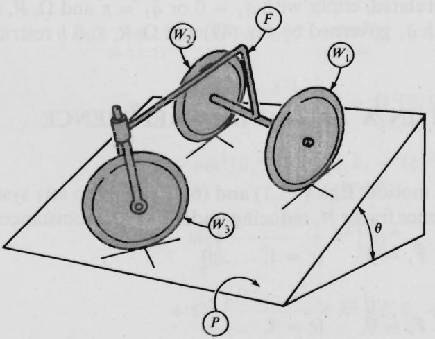
Figure 6.5.1

q_{6}\triangleq\mathbf{p}^{*}\cdot\mathbf{n}_{1}\qquad q_{7}\triangleq\mathbf{p}^{*}\cdot\mathbf{n}_{2}

where \mathbf{p}^{*} is thepositionvectorfrom a point o fixed in P to themasscenter S^{*} of s , and \mathbf{n}_{1} and \mathbf{n}_{2} are, respectively, a horizontal unit vector and a unit vector pointingin the direction of steepest descent on P asindicatedin Fig.6.5.2 Generalized speeds u_{1},\dotsc,u_{7} may be defined as

u_{1}\triangleq\dot{q}_{3}\qquad u_{2}\triangleq\dot{q}_{4}\qquad u_{3}\triangleq\dot{q}_{5}

u_{4}\triangleq\dot{q}_{1}\qquad u_{5}\triangleq\dot{q}_{2}\qquad u_{6}\triangleq\mathbf{v}^{*}\cdot\mathbf{f}_{1}\qquad u_{7}\triangleq\mathbf{v}^{*}\cdot\mathbf{f}_{2}

where \mathbf{v}^{*} is thevelocity of S^{*} ,and \mathbf{f}_{1} and \mathbf{f}_{2} are unit vectors directed as indicated in Fig. 6.5.2.

On the basis of the assumption that W_{1},\,W_{2} and W_{3} roll,rather than slip, on P ,equations are to be formulated for the purpose of determining how T is related totheinclination angle \theta the total mass M of s the dimensions R,a,b and L (see Fig. 6.5.2), and the generalized coordinates q_{1},\dots,q_{7} when \boldsymbol{s} is at rest.

The assumption that W_{1} W_{2} ,and W_{3} donotslipon P leadstofive motion constraint equations (see Sec. 2.13). Hence, S possessestwodegrees of freedom, and Eqs. (1) can be written with p=2 . To form \tilde{F} (r=1,2) wewrite

\tilde{F}_{r}\underset{(4.6\cdot1)}{=}M g\mathbf{k}\cdot\tilde{\mathbf{v}}_{r}^{\ *}\,+\,T\mathbf{f}_{2}\cdot\tilde{\mathbf{o}}_{r}^{\ F}-\,T\mathbf{f}_{2}\cdot\tilde{\mathbf{o}}_{r}^{\ W_{2}}\qquad(r=1,2)

where \mathbf{k} isa unit vector directed verticallydownward;thatiswith \mathbf{f}_{3}\triangleq\mathbf{f}_{1}\times\mathbf{f}_{2}

{\bf k}=\sin q_{s}\sin\theta{\bf f}_{1}+\cos q_{s}\sin\theta{\bf f}_{2}-\cos\theta{\bf f}_{3}

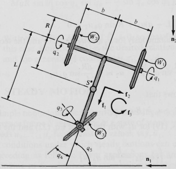
The partial velocities and partial angular velocities appearing in Eqs. (10) are found as follows.

The velocities of the points of W_{1},\,W_{2} ,and W_{3} that are in contact with P must be equal to zero. In the case of W_{1} , this requirement can be expressed as [use Eq. (2.7.1) twice]

\mathbf{v^{*}}+\mathbf{\Delta}\mathbf{\omega}\mathbf{^{F}}\times(-a\mathbf{f}_{1}+b\mathbf{f}_{2})+\mathbf{\omega}\mathbf{^{W_{1}}}\times(-R\mathbf{f}_{3})=0

where

\mathbf{\omega}\mathbf{\sigma}\mathbf{\omega}\mathbf{\omega}\mathbf{\omega}\mathbf{\omega}\mathbf{\omega}\mathbf{\omega}\mathbf{\omega}\mathbf{\omega}\mathbf{\omega}\mathbf{\omega}

and

\begin{array}{r l r}{{\bf\omega0}^{W_{1}}}&{=}&{{\bf\omega0}^{F}+\,\dot{q}_{1}{\bf f}_{2}=u_{3}\,{\bf f}_{3}+u_{4}\,{\bf f}_{2}}\end{array}

Moreover,

\mathbf{v}^{*}=u_{6}\mathbf{f}_{1}+u_{7}\mathbf{f}_{2}

Hence,

(u_{6}-b u_{3}-R u_{4})\mathbf{f}_{1}+(u_{7}-a u_{3})\mathbf{f}_{2}\,=\,0

which means that

u_{6}-b u_{3}-R u_{4}=0\qquad u_{7}-a u_{3}=0

Proceeding similarly in connection with W_{2} and W_{3} , one finds that

\begin{array}{r}{\mathbf{\omega}_{0}^{\omega^{W_{2}}}=u_{3}\mathbf{f}_{3}+u_{5}\mathbf{f}_{2}\qquad\mathbf{\omega}_{0}^{\omega^{W_{3}}}=(u_{3}-u_{2})\mathbf{f}_{3}+u_{1}(\sin q_{4}\mathbf{f}_{1}+\cos q_{4}\mathbf{f}_{2})}\end{array}

and that, in addition to Eqs. (17), the motion constraint equations

u_{6}+b u_{3}-R u_{5}=0\qquad u_{6}-R\cos q_{4}u_{1}=0

and

u_{7}+(L-a)u_{3}+R\sin q_{4}u_{1}=0

must be satisfied. Solved simultaneously for u_{3} and \pmb{u}_{7} , Eq. (20) and the second of Eqs. (17) yield

u_{3}=-\,\frac{R}{L}\mathrm{sin}\;q_{4}u_{1}\qquad u_{7}=-\,\frac{a R}{L}\mathrm{sin}\;q_{4}u_{1}

The second of Eqs. (19) shows that

u_{6}=R\cos q_{4}u_{1}

and, solving the first of Eqs. (19) for \pmb{u}_{5} with the aid of Eq. (22) and the first of Eqs. (21), one obtains

u_{5}=\biggl(\cos q_{4}-\frac{b}{L}\sin q_{4}\biggr)u_{1}

Hence,

\begin{array}{l}{{{\displaystyle{\bf v}^{*}\;=\;R\,\cos q_{4}u_{1}{\bf f}_{1}\,-\frac{a R}{L}{\sin q_{4}u_{1}{\bf f}_{2}}}\displaystyle{}}}\\ {{{\displaystyle({}^{15})\qquad\quad({}^{22})}\displaystyle{}}}\\ {{{\displaystyle{\bf o}^{F}\;=\;-\,\frac{R}{L}{\sin q_{4}u_{1}{\bf f}_{3}}}}}\end{array}

and

\mathbf{\omega}\mathbf{\omega}^{W_{2}}=-\frac{R}{L}\sin{{q_{4}}u_{1}}\mathbf{f}_{3}+\biggl(\cos{{q_{4}}}-\frac{b}{L}\sin{{q_{4}}}\biggr)u_{1}\mathbf{f}_{2}

The partial velocities of s^{*} and the partial angular velocities of {\pmb F} and W_{2} needed for substitution into Eqs. (10) thus are given by [see Eqs. (24)-(26)]

\begin{array}{l}{{\displaystyle{\widetilde{\bf v}_{1}}^{*}=R\cos q_{4}{\bf f}_{1}-\frac{a R}{L}\sin q_{4}{\bf f}_{2}}\ ~}\\ {{\displaystyle}}\\ {{\displaystyle{\widetilde{\bf\Phi}_{1}}^{F}=\mathrm{~-~}\frac{R}{L}\sin q_{4}{\bf f}_{3}}}\end{array}

{\tilde{\bf\Phi}}_{1}{}^{W_{2}}=\left(\cos q_{4}-\frac{b}{L}\sin q_{4}\right){\bf f}_{2}-\frac{R}{L}\sin q_{4}{\bf f}_{3}

and

\tilde{\mathbf{v}}_{2}{}^{*}=\tilde{\omega}_{2}{}^{F}=\tilde{\omega}_{2}{}^{W_{2}}=0

Substituting these into Eqs. (10) with r=1 , and setting the result equal to zero in accordance with Eqs. (1), one finds with the aid of Eq. (11) that

M g R\,\sin\,\theta\biggl(\cos q_{4}\,\sin\,q_{5}-\frac{a}{L}\sin\,q_{4}\,\cos q_{5}\biggr)\,-\,T\biggl(\cos q_{4}-\frac{b}{L}\sin q_{4}\biggr)=0

With r=2\AA ,Eqs. (10) yield \widetilde{F}_{2}=0 , so that Eqs. (1) are satisfied identically in this case. Equation (31) is the desired relationship between T,\theta,M,R,a,b,L, and the generalized coordinates q_{1},\ldots,q_{7}

6.6 STEADY MOTION

A simple nonholonomic system S possessing \pmb{p} degrees of freedom in a Newtonian reference frame N is said to be in a state of steady motion in N when the generalized speeds u_{1},\dotsc,u_{p} have constant values, say, \bar{u}_{1},...,\bar{u}_{p} , respectively. To determine the conditions under which steady motions can occur, use Eqs. (6.1.1) or (6.1.2), proceeding as follows: Form expressions for angular velocities of rigid bodies belonging to \pmb{S}, velocities of mass centers of these bodies, and so forth, without regard to the fact that u_{1},\dotsc,u_{p} are to remain constant, and use these expressions to construct partial angular velocities and partial velocities. Set u_{r}=\bar{u}_{r}(r=1,\ldots,p) in angular velocity and velocity expressions, then differentiate with respect to time to generate needed angular accelerations of rigid bodies and accelerations of various points.Formulate expressions for {\widetilde{\boldsymbol{F}}}, and \tilde{F}_{r}^{\mathrm{~*~}}(r=1,\dotsc,p) in the case of Eqs. (6.1.1), or F_{r} and F_{r}^{\ast}\left(r=1,\ldots,n\right) in the case of Eqs. (6.1.2), and substitute into Eqs. (6.1.1) or (6.1.2).

Example Figure 6.6.1 shows a right-circular, uniform, solid cone C in contact with a fixed, horizontal plane P The motion that C performs-when C rolls on P in such a way that the mass center C^{*} of C (see Fig. 6.6.1) remains fixed while theplane determinedby the axis of C and a verticai line passing through C^{*} has an angular velocity -\Omega\mathbf{k} \Omega constant)--is a steady motion, as will be shown presently. But this motion can take place only if \Omega , the radius R of the base of C ,theheight 4h of C ,and the inclination angle \theta (see Fig. 6.6.1) are related to each other suitably.To determine the conditionsunderwhich the motion is possible, we begin by noting that C has three degrees of freedom, and introduce generalized speeds u_{1},u_{2} , and u_{3} as

u_{r}\triangleq\mathbf{\omega}\cdot\mathbf{b},\qquad(r=1,2,3)

where \mathbf{\omega_{60}} is the angular velocity of C , and \ensuremath{\mathbf{b}}_{1},\,\ensuremath{\mathbf{b}}_{2} , and {\bf b}_{3} aremutually perpendicular unit vectors directed as indicated in Fig. 6.6.1. (Note that {\bf b}_{2} and {\bf b}_{3} are not fixed in C

As is pointed out in Problem 3.12, \mathbf{\omega_{60}} is given by

\mathbf{0}=\Omega\mathrm{s}\theta{\left(\frac{h}{R}\,\mathbf{b}_{1}+\mathbf{b}_{2}\right)}

when C moves as required. Hence, u_{1},u_{2} ,and u_{3} then have the constant values

\bar{u}_{1}=\Omega s\theta\,\frac{h}{R}\qquad\bar{u}_{2}=\Omega s\theta\qquad\bar{u}_{3}=0

respectively.

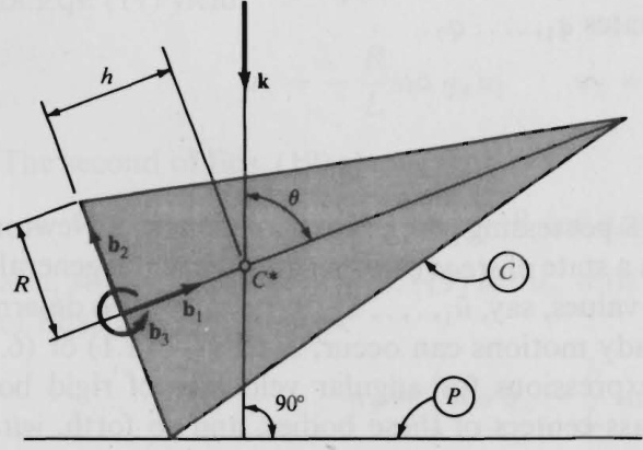
Figure 6.6.1

The generalized active forces {\widetilde{\boldsymbol{F}}}, (r=1,2,3) are expressed most conveniently as

\tilde{F}_{r}\mathop{=}_{(4.8.2)}M g{\bf k}\cdot\tilde{\bf v}_{r}^{\mathrm{~*~}}\qquad(r=1,2,3)

where M is the mass of c and

\mathbf{k}=\mathbf{\mu}-(\mathbf{c}\theta\mathbf{b}_{1}+\mathbf{s}\theta\mathbf{b}_{2})

As for the generalized inertia forces \widetilde{F}_{r}{}^{*}\left(r=1,2,3\right) ,we write

\tilde{F}_{r_{\ (4.11.7)}}^{*}\tilde{\upomega}_{r}\cdot{\bf T}^{*}\,+\,\tilde{\upnu}_{r}^{\ *}\cdot{\bf R}^{*}\qquad(r=1,2,3)

and defer detailed consideration of \mathbf{T}^{*} and \mathbf{R}^{\ast} until after expressions for \tilde{\mathbf{o}}_{r} and \tilde{\mathbf{v}}_{r}^{\star} have been constructed.

From Eqs. (1),

\mathbf{\omega}\mathbf{\omega}\mathbf{\omega}\mathbf{\omega}\mathbf{\omega}\mathbf{\omega}\mathbf{\omega}\mathbf{\omega}\mathbf{\omega}\mathbf{\omega}\mathbf{\omega}\mathbf{\omega}\mathbf{\omega}\mathbf{u}_{1}\mathbf{b}_{1}\mathbf{\beta}+u_{2}\mathbf{\omega}\mathbf{b}_{2}+u_{3}\mathbf{b}_{3}

and, when c rolls on \pmb{P} , the velocity \mathbf{v^{*}} of C^{\ast} is given by

\begin{array}{r l}&{\mathbf{v^{*}}=\mathbf{\omega}\times(h\mathbf{b}_{1}+R\mathbf{b}_{2})}\\ &{\quad=-R u_{3}\mathbf{b}_{1}+h u_{3}\mathbf{b}_{2}+(R u_{1}-h u_{2})\mathbf{b}_{3}}\\ &{\quad(7)}\end{array}

The partial angular velocities and partial velocities obtained by inspection of Eqs. (7) and (8), respectively, are recorded in Table 6.6.1.

The steady motion form of \mathbf{\delta} is available in Eq. (2). Differentiating both sides of this equation with respect to time in order to find \pmb{\alpha}, theangular accelerationof c weobtain

{\mathfrak{a}}=\mathfrak{w}^{B}\times\left[\Omega\mathrm{s}\theta\bigg(\frac{h}{R}\,\mathfrak{b}_{1}+\mathfrak{b}_{2}\bigg)\right]

where \mathbf{e}\mathbf{\mathrm{{s}}}^{B} , the angular velocity of a reference frame in which \ensuremath{\mathbf{b}}_{1},\,\ensuremath{\mathbf{b}}_{2} ,and {\bf b}_{3} are fixed, is given by

\mathbf{\omega}\mathbf{\omega}^{B}=\Omega(\mathbf{c}\theta\mathbf{b}_{1}+\mathbf{\omega}\mathbf{s}\theta\mathbf{b}_{2})

Consequently,

\alpha\underset{(9,10)}{=}\Omega^{2}\mathrm{s}\theta\bigg(\mathrm{c}\theta-\frac{h}{R}\,\mathrm{s}\theta\bigg)\mathbf{b}_{3}

Table 6.6.1

<html>

	'?
1	b1 Rb3
2	b2 -hb3
3	b3 -Rb, + hb2

</html>

The velocity \mathbf{v^{*}} is equal to zero, by hypothesis, during the steady motion of interest, a result one can verify by setting u_{r}=\bar{u}_{r} (r=1,2,3) in Eq. (8) and then using Eqs. (3). It follows that {\mathbf z}^{\ast} , the acceleration of C^{\ast} , vanishes, and this means that the inertia force \mathbf{R}^{\ast} appearing in Eqs. (6) also vanishes. As for the inertia torque \mathbf{T^{*}} , one can express this as

\mathbf{T}^{*}=\Omega^{2}\mathrm{s}\theta\bigg(I_{1}\frac{h}{R}\mathrm{s}\theta-I_{2}\mathrm{c}\theta\bigg)\mathbf{b}_{3}

by substituting from Eqs. (11) and (2) into Eq. (4.11.8), with

\mathbf{I}=I_{1}\mathbf{b}_{1}\mathbf{b}_{1}+I_{2}(\mathbf{b}_{2}\mathbf{b}_{2}+\mathbf{b}_{3}\mathbf{b}_{3})

Expressed in terms of M,R , and \pmb{h} the moments of inertia I_{1} and I_{2} are given by (see Appendix I)

I_{1}=\frac{3M R^{2}}{10}\qquad I_{2}=\frac{3M(R^{2}+4h^{2})}{20}

Referring to Eq. (5) and Table 6.6.1, one finds by substitution into Eqs (4) that

\tilde{F}_{1}=\tilde{F}_{2}=0\qquad\tilde{F}_{3}=M g(R\mathrm{c}\theta-h\mathrm{s}\theta)

Similarly, Eqs. (6) lead to

\widetilde{F}_{1}{}^{*}=\widetilde{F}_{2}{}^{*}=0\qquad\widetilde{F}_{3}{}^{*}=\Omega^{2}\mathsf{s}\theta\bigg(I_{1}\,\frac{h}{R}\mathsf{s}\theta-I_{2}\mathsf{c}\theta\bigg)

Consequently, Eqs. (1) are satisfied identically when r=1 and r=2 ;for r=3\cdot , substitution from Eqs. (15), (16), and (14) into Eqs. (1) leads to the conclusion that the steady motion under consideration can take place only when

\frac{3}{20}\left(\frac{R\Omega^{2}}{g}\right)\left\{\left[1\,+\,4\left(\frac{h}{R}\right)^{2}\right]\mathrm{c}\theta\,-\,2\left(\frac{h}{R}\right)\mathrm{s}\theta\right\}\mathrm{s}\theta\,+\frac{h}{R}\mathrm{s}\theta\,-\,\mathrm{c}\theta\,=\,0

6.7 MOTIONS RESEMBLING STATES OF REST

A simple nonholonomic system S possessing \pmb{p} degrees of freedom in a Newtonian reference frame N is said to be performing a motion resembling a state of rest when the generalized coordinates q_{1},\ldots,q_{n} have constant values, say, \bar{q}_{1},\ldots,\bar{q}_{n} respectively. To determine the conditions under which such motions are possible, one can use Eqs. (6.1.1) or (6.1.2), employing a procedure analogous to that set forth in Sec. 6.6. Alternatively, if the kinetic energy K , when regarded as a function of q_{1},\ldots,q_{n},\,\dot{q}_{1},\ldots,\dot{q}_{n} and t_{\mathrm{:}} does not involve t explicitly, then one can use the equations

\sum_{s=1}^{n}\frac{\partial K}{\partial q_{s}}\left(W_{s r}+\sum_{k=p+1}^{n}\,W_{s k}\,A_{k r}\right)\,+\,\widetilde{F}_{r}=0\qquad(r=1,\ldots,p)

where W_{s r}\left(s=1,\ldots,n;r=1,\ldots,p\right) and A_{k r}\left(k=p+1,\ldots,n;r=1,\ldots,p\right) have the same meanings as in Eqs. (2.14.5) and (2.13.1), respectively, and \tilde{F}_{r}\,(r=1,\ldots,\,p) are defined in Eqs. (4.4.1). If u_{1},\ldots,u_{n} are defined as u_{r}=\dot{q}_{r}\,(r=1,\dots,n), then Eqs. (1) give way to

\frac{\partial K}{\partial q_{r}}+\sum_{s=p+1}^{n}\frac{\partial K}{\partial q_{s}}C_{s r}+\widetilde{F}_{r}=0\qquad(r=1,\ldots,p)

where C_{s r}\left(s=p+1,\ldots,n;r=1,\ldots,p\right) has the same meaning as in Eq. (5.1.13). If s is a holonomic system with u_{r} defined as in Eqs. (2.12.1), so that Eqs. (2.14.5) apply, then

\sum_{s=1}^{n}\frac{\partial K}{\partial q_{s}}\,W_{s r}+F_{r}=0\qquad(r=1,\ldots,n)

during motions resembling states of rest; and if u_{r}=\dot{q}_{r}\,(r=1,\dots,n) ,then Eqs. (3) are replaced with

\frac{\partial K}{\partial q_{r}}+F_{r}=0\qquad(r=1,\ldots,n)

When using Eqs. (1)-(4), one can work with expressions for K,\tilde{F}_{r}(r=1,\dots,p), or F, (r=1,\ldots,n) that apply only when {\dot{q}}_{1}=\dots={\dot{q}}_{n}=0, rather than during the most general motion of s ; generally, this simplifies matters considerably.

If s possesses a potential energy V in N ,and \mathscr{L} is defined as

{\mathcal{L}}\triangleq K-V

then Eqs. (1)-(4) can be replaced with

{\begin{array}{r l}{\displaystyle\sum_{s=1}^{n}{\frac{\partial{\mathcal{L}}}{\partial q_{s}}}\left(W_{s r}+\sum_{k=p+1}^{n}W_{s k}A_{k r}\right)=0\quad}&{(r=1,\ldots,p)}\\ {\displaystyle{\frac{\partial{\mathcal{L}}}{\partial q_{r}}}+\sum_{s=p+1}^{n}{\frac{\partial{\mathcal{L}}}{\partial q_{s}}}C_{s r}=0\quad}&{(r=1,\ldots,p)}\\ {\displaystyle\sum_{s=1}^{n}{\frac{\partial{\mathcal{L}}}{\partial q_{s}}}W_{s r}=0\quad}&{(r=1,\ldots,n)}\\ {\displaystyle{\frac{\partial{\mathcal{L}}}{\partial q_{r}}}=0\quad}&{(r=1,\ldots,n)}\end{array}}

respectively. Use of these equations obviates forming expressions for accelerations.

Derivations If K , when regarded as a function of q_{1},\ldots,q_{n} ， {\dot{q}}_{1},\dots,{\dot{q}}_{n} , and t does not involve t explicitly, then the partial derivatives \partial K/\partial{\dot{q}}_{r} (r=1,\ldots,n) are functions f_{r}\left(r=1,\ldots,n\right) of precisely the _{2n} variables q_{r} and {\dot{q}}, (r\!=1,\ldots,n) ， so that one can write

{\frac{\partial K}{\partial{\dot{q}}_{r}}}=f_{r}(q_{1},\dots,q_{n},{\dot{q}}_{1},\dots,{\dot{q}}_{n})\qquad(r=1,\dots,n)

and

{\frac{d}{d t}}\left({\frac{\partial K}{\partial{\dot{q}}_{r}}}\right)=\sum_{s=1}^{n}\left({\frac{\partial f_{r}}{\partial q_{s}}}{\dot{q}}_{s}+{\frac{\partial f_{r}}{\partial{\dot{q}}_{s}}}{\ddot{q}}_{s}\right)\qquad(r=1,\ldots,n)

But, since q_{s}=\bar{q}_{s}\,(s=1,\dots,n) by hypothesis,

{\dot{q}}_{s}={\ddot{q}}_{s}=0\qquad(s=1,\dots,n)

sothat

\frac{d}{d t}\left(\frac{\partial K}{\partial{\dot{q}}_{r}}\right)_{(11,12)}0~~~~~(r=1,\dots,n)

and use of these relationships in conjunction with the four equations in Problem 11.12 (taken in reverse order) leads directly to Eqs. (1)-(4).

When s possesses apotential energy V in N \widetilde{F}_{r} in Eqs. (1) can be replaced with the right-hand member of Eq. (5.1.18), which shows that

\sum_{s=1}^{n}\left({\frac{\partial K}{\partial q_{s}}}-{\frac{\partial V}{\partial q_{s}}}\right)\left(W_{s r}+\sum_{k=p1}^{n}W_{s k}A_{k r}\right)=0\qquad(r=1,\ldots,p)

under these circumstances.Now,

{\frac{\partial K}{\partial q_{s}}}-{\frac{\partial V}{\partial q_{s}}}={\frac{\partial}{\partial q_{s}}}(K-V)={\frac{\partial{\mathcal{L}}}{\partial q_{s}}}\qquad(s=1,\ldots,n)

Substitution from Eqs. (15) into Eqs. (14) produces Eqs. (6). Similarly, Eqs. (2), (15), and (5.1.14) lead to Eqs. (7); Eqs. (3), (15), and (5.1.9) underlie Eqs. (8); and Eqs. (4), (15), and (5.1.2) can be used to establish the validity of Eqs. (9).

Example Two uniform bars, A and B ,each of mass m and length L , are connected by a pin, and A ispinned toavertical shaft thatismade torotatewith constant angular speed \Omega as indicated in Fig. 6.7.1. (The axes of the pins are

Figure 6.7.1

parallel to each other and horizontal.) This system can move in such a way that q_{1} and q_{2} (see Fig. 6.7.1) remain constant. Equations (9) will be used to formulate equations governing q_{1} and q_{2} during such motions.

When \dot{q}_{1}=\dot{q}_{2}=0, the angular velocities of A and \textbf{\emph{B}} can be written

\mathbf{\omega}\mathbf{\omega}^{\mathbf{4}}=\mathbf{\omega}-\Omega(\mathbf{\mathsf{s}}_{1}\mathbf{\mathsf{a}}_{1}+\mathbf{\mathsf{c}}_{1}\mathbf{\mathsf{a}}_{2})\qquad\mathbf{\omega}\mathbf{\omega}^{\mathbf{B}}=\mathbf{\omega}-\Omega(\mathbf{\mathsf{s}}_{2}\mathbf{\mathsf{b}}_{1}+\mathbf{\mathsf{c}}_{2}\mathbf{\,}\mathbf{\mathsf{b}}_{2})

where {\mathbf{a}}_{i} and {\mathfrak{b}}_{i}\,(i=1,2) are unit vectors directed as shown in Fig. 6.7.1; the velocityof B^{*} ,themasscenterof \textbf{\emph{B}} is

\mathbf{v}^{B^{*}}=L\Omega\left(s_{1}+\frac{s_{2}}{2}\right)\mathbf{b}_{3}

and the kinetic energy K is thus given by

\begin{array}{l}{{{\cal K}=\displaystyle\frac{1}{2}\frac{m L^{2}}{3}\,\Omega^{2}{s_{1}}^{2}\ \ \ +\ \ \ \ \frac{1}{2}\frac{m L^{2}}{12}\ \,\Omega^{2}{s_{2}}^{2}+\displaystyle\frac{1}{2}m L^{2}\Omega^{2}\biggl(s_{1}+\frac{s_{2}}{2}\biggr)^{2}}}\\ {{\mathrm{\large~(Problem~10.4,16)~}\,(s.4.2)\qquad\ \ (5.4.7.16)\qquad\qquad\ \ (5.4.4,17)}}\\ {{\mathrm{\large~=\displaystyle\frac{mL^{2}\Omega^{2}}{2}\left(\frac{4}{3}s_{1}^{\ 2}+s_{1}s_{2}+\frac{1}{3}s_{2}^{\ 2}\right)}}}\end{array}

The potential energy V can be expressed as

V=\,-m g L\left(\frac{1}{2}\mathtt{c}_{1}+\mathtt{c}_{1}+\frac{1}{2}\mathtt{c}_{2}\right)=\,-\,\frac{m g L}{2}(3\mathtt{c}_{1}+\mathtt{c}_{2})\ \ \ \ .

Consequently,

{\mathcal{L}}={\frac{m L^{2}{\Omega}^{2}}{2}}{\left({\frac{4}{3}}\,{s_{1}}^{2}+\,{s_{1}}{s_{2}}\,+{\frac{1}{3}}\,{s_{2}}^{2}\right)}+{\frac{m g L}{2}}(3{\bf c}_{1}\,+\,{\bf c}_{2})

and, setting \partial\mathcal{L}/\partial q_{r}=0\,(r=1,2) , one obtains the desired equations, namely,

\left(\frac{L\Omega^{2}}{g}\right){\bf c}_{1}(8{\bf s}_{1}\,+\,3{\bf s}_{2})\,-\,9{\bf s}_{1}=0

and

\left(\frac{L\Omega^{2}}{g}\right)\mathsf{c}_{2}(3\mathsf{s}_{1}+2\mathsf{s}_{2})-3\mathsf{s}_{2}=0

EXTRACTION OF INFORMATION FROM EQUATIONS OFMOTION

This chapter is intended to bring to fruition the effort that has been expended by the reader in learning the material covered in the first six chapters. Following the introduction, in Sec. 7.1, of terminology employed in connection with solutions of equations of motion, several theorems that permit the construction of integrals of equations of motion are presented in Secs. 7.2 and 7.3. Exact closed-form solutions are considered in Sec. 7.4, and means for obtaining numerical results when closed-form solutions are unavailable are discussed in Sec. 7.5. These techniques, used in conjunction with material in Sec. 6.3, permit the evaluation of constraint forces and constraint torques, as is shown in Sec. 7.6. Section 7.7 deals with a purely mathematical problem that arises frequently in dynamics, namely, finding real solutions of a set of nonlinear, nondifferential equations. The concepts of generalized impulse and generalized momentum are introduced in Sec. 7.8 in preparation for the presentation, in Sec. 7.9, of a method for analyzing phenomena involving collisions. Finally, Sec. 7.10 contains an exposition of the principal concepts underlying the theory of small vibrations of mechanical systems.

7.1 INTEGRALS OF EQUATIONS OF MOTION

The behavior of a simple nonholonomic system S possessing \pmb{p} degrees of freedom in a Newtonian reference frame N (see Sec. 2.13) is governed by _{2n} equations called, collectively, the equations of motion of s in N . This set of equations consists of three subsets: the n kinematical differential equations, Eqs. (2.12.1) or, equivalently, Eqs. (2.14.5); the n-p nonholonomic constraint equations, Eqs. (2.13.1); and the \pmb{p} dynamical differential equations, Eqs. (6.1.1). If s is a holonomic system, then n=p , the nonholonomic constraint equations are absent, and Eqs. (6.1.2) furnish n dynamical equations.

A solution of the equations of motion is said to be in hand when the generalized coordinates q_{1},\ldots,q_{n} (see Sec. 2.10) and generalized speeds u_{1},\ldots,u_{n} (see Sec. 2.12) are known as functions of the time t, The general solution of the equations of motion consists of _{2n} independent equations of the form

f_{i}\left(q_{1},\dots,q_{n},u_{1},\dots,u_{n},t\right)=C_{i}\qquad(i=1,\dots,2n)

where f_{i}\,(i=1,\ldots,2n) is a function whose total time-derivative vanishes, whenever q_{1},\ldots,q_{n} and u_{1},\ldots,u_{n} satisfy all equations of motion, and C_{1},...,C_{2n} are arbitrary constants. An equation having the form of Eqs. (1) is called an integral of the equations of motion. Thus, the general solution of the equations of motion consists of _{2n} integrals.

Examples For the nonholonomic system s formed by the particle \boldsymbol{P}_{1} and the sharp-edged circular disk \pmb{D} connected by a rigid rod \pmb R as in the example in Sec. 2.13, \pmb{p}=2 and n=3 When the kinematical differential equations are taken to be [see Eqs. (2.12.7)]

u_{1}=\dot{q}_{1}\mathsf{c}_{3}+\dot{q}_{2}\mathsf{s}_{3}\qquad u_{2}=-\dot{q}_{1}\mathsf{s}_{3}+\dot{q}_{2}\mathsf{c}_{3}\qquad u_{3}=\dot{q}_{3}

then the nonholonomic constraint equation expressing the restriction that the center of \pmb{D} may not move perpendicularly to \pmb R is [see Eq. (2.13.12)]

u_{3}=-\,\frac{u_{2}}{L}

Furthermore, if line \pmb{Y} in Fig. 2.13.1 is vertical, \boldsymbol{P}_{1} and \pmb{D} have masses m_{1} and m_{2} , respectively, and \boldsymbol{P}_{1} is subjected to the action of a contact force \mathbf{K} given by Eq. (5.1.26), then the generalized active forces for s are given by [see Eqs. (5.1.39)]

\begin{array}{l}{{\displaystyle{\widetilde{F}_{1}=k-(m_{1}+m_{2})g s_{3}}}}\\ {{\displaystyle{\widetilde{F}_{2}=\frac{k}{L}(q_{1}s_{3}-q_{2}c_{3})-m_{1}g c_{3}}}}\end{array}

while the generalized inertia forces can be written (see Problem 8.16)

\begin{array}{r l}&{\tilde{F}_{1}^{*}=(m_{1}+m_{2})(\omega^{2}q_{1}\mathsf{c}_{3}-\dot{u}_{1})-\frac{{m_{1}}{u_{2}}^{2}}{L}+m_{2}L\omega^{2}\mathsf{c}_{3}^{2}}\\ &{\qquad\qquad\qquad\qquad\qquad\qquad\qquad\qquad\qquad}\\ &{\tilde{F}_{2}^{*}=\,-m_{1}\bigg(\dot{u}_{2}+\omega^{2}q_{1}\mathsf{s}_{3}-\frac{u_{1}u_{2}}{L}\bigg)}\end{array}

Substitution from Eqs. (4)-(7) into Eqs. (6.1.1) thus yields the dynamical differential equations

k-(m_{1\atop(4)}+m_{2})g s_{3}+(m_{1}+m_{2})(\omega^{2}q_{1}c_{3}-\dot{u}_{1})-\frac{m_{1}{u_{2}}^{2}}{L}+m_{2}L\omega^{2}{c_{3}}^{2}=0

and

\frac{k}{L}(q_{1}\mathsf{s}_{3}-q_{2}\mathsf{c}_{3})-m_{1}g\mathsf{c}_{3}-m_{1}\left(\dot{u}_{2}+\omega^{2}q_{1}\mathsf{s}_{3}-\frac{u_{1}u_{2}}{L}\right)=0

Equations (2), (3), (8), and (9) are the six equations of motion of s

As will be shown presently, the equation

\begin{array}{r}{-k(q_{1}\mathsf{c}_{3}+q_{2}\mathsf{s}_{3})+g[(m_{1}+m_{2})q_{2}+m_{2}L\mathsf{s}_{3}]+\frac{1}{2}[(m_{1}+m_{2}){u_{1}}^{2}+m_{1}{u_{2}}^{2}]}\\ {-\frac{1}{2}\omega^{2}[m_{1}{q_{1}}^{2}+m_{2}(q_{1}+\,L\mathsf{c}_{3})^{2}]=C\quad(10)}\end{array}

where C is an arbitrary constant, is an integral of the equations of motion of S. It does not matter for present purposes how this integral was found; this subject is discussed in its own right in the example in Sec. 7.2.

Denoting the left-hand member of Eq. (10) by f(q_{1},q_{2},q_{3},u_{1},u_{2},u_{3},t), and expressing the total time-derivative of f as

{\dot{f}}=\sum_{r=1}^{3}\left({\frac{\partial f}{\partial q_{r}}}{\dot{q}}_{r}+{\frac{\partial f}{\partial u_{r}}}{\dot{u}}_{r}\right)+{\frac{\partial f}{\partial t}}

one finds that

\begin{array}{r l}{\dot{f}_{(11,10)}-\{-k c_{3}-\ \omega^{2}[m_{1}q_{1}+m_{2}(q_{1}+L c_{3})]\}\dot{q}_{1}}&{}\\ {\dot{+}\left[-k s_{3}+g(m_{1}+m_{2})\right]\dot{q}_{2}}&{}\\ {\dot{+}\left[k(q_{1}s_{3}-q_{2}c_{3})+g m_{2}L c_{3}+\omega^{2}m_{2}(q_{1}+L c_{3})L s_{3}\right]\dot{q}_{3}}&{}\\ {\dot{+}\left(m_{1}+m_{2})u_{1}\dot{u}_{1}+m_{1}u_{2}\dot{u}_{2}}&{}\end{array}

Solution of the kinematical differential equations, Eqs. (2), for {\dot{q}}_{1},{\dot{q}}_{2} , and \dot{\boldsymbol{q}}_{3} yields

{\dot{q}}_{1}=u_{1}{\mathsf{c}}_{3}-u_{2}{\mathsf{s}}_{3}\qquad{\dot{q}}_{2}=u_{1}{\mathsf{s}}_{3}+u_{2}{\mathsf{c}}_{3}\qquad{\dot{q}}_{3}=u_{3}

while solution of the dynamical diferential equations for \dot{u}_{1} and \dot{u}_{2} leads to

\begin{array}{l}{{\dot{u}_{1}=\omega^{2}\mathbf{c}_{3}\left(q_{1}+\displaystyle\frac{m_{2}L\mathbf{c}_{3}}{m_{1}+m_{2}}\right)+\displaystyle\frac{k}{m_{1}+m_{2}}-g\mathbf{s}_{3}-\displaystyle\frac{m_{1}{u_{2}}^{2}}{(m_{1}+m_{2})L}}}\\ {{\dot{u}_{2}=-\omega^{2}q_{1}\mathbf{s}_{3}+\displaystyle\frac{k}{m_{1}L}(q_{1}\mathbf{s}_{3}-q_{2}\mathbf{c}_{3})-g\mathbf{c}_{3}+\displaystyle\frac{u_{1}u_{2}}{L}}}\end{array}

If \pmb{u}_{3} in the third of Eqs. (13) now is replaced with -u_{2}/L in accordance with the nonholonomic constraint equation, Eq. (3), and Eqs. (13)-(15) then are used to eliminate {\dot{q}}_{1},\,{\dot{q}}_{2},\,{\dot{q}}_{3},\,{\dot{u}}_{1} , and \dot{u}_{2} from Eq. (12), \boldsymbol{\hat{f}} is found to be equal to zero, and this establishes Eq. (10) as an integral of the equations of motion of S. (To obtain the general solution of the equations of motion, one must produce five more integrals.)

As a second example, we consider a system governed by differential equations whose explicit solution is well known, namely, the harmonic oscillator, that is, any system whose behavior is governed by the differential equation

\ddot{q}+\omega^{2}q=0

where \omega^{2} is a constant. This equation can be replaced with the two firstorder equations

\dot{q}=u\qquad\dot{u}=-\omega^{2}q

the first of which is simply a definition of \pmb{u} and plays the role of a kinematical differential equation, while the second is a dynamical differential equation. Thus, n=p=1

Using the same procedure as in the preceding example, one can verify that

q\sin\omega t+{\frac{u}{\omega}}\cos\omega t=C_{1}

and

q\cos\omega t-{\frac{u}{\omega}}\sin\omega t=C_{2}

are integrals of the equations of motion, Eqs. (17). Together, these two integrals constitute the general solution of Eqs. (17). To bring this solution into a form that may be more familiar, one can solve Eq. (18) for {\pmb u}/\omega substitute the result into Eq. (19), and obtain, after simplification,

q=C_{1}\,\sin\omega t+C_{2}\cos\omega t

7.2 THE ENERGY INTEGRAL

When a system S possesses a potential energy V in a Newtonian reference frame N (see Sec. 5.1), there may exist an integral of the equations of motion of s in N (see Sec. 7.1) that can be expressed as

H=C

where c is a constant and \pmb{H} , called the Hamiltonian of \boldsymbol{s} in N , is defined as

H\triangleq V+K_{2}-K_{0}

with \pmb{K}_{0} and K_{2} given by Eqs. (5.5.7) and (5.5.9), respectively. Equation (1) is called the energy integral of the equations of motion of \boldsymbol{s} in N .The conditions under which it exists depend on the manner in which generalized speeds are introduced and on whether \boldsymbol{s} is a holonomic or nonholonomic system. In Table 7.2.1, sufficient conditions for the existence of the energy integral of S in N are indicated by listing the numbers of equations satisfaction of which ensures the existence of an energy integral.

Table 7.2.1

<html>

u,=q	X,=0, Ws=0s	u, = ∑ Ysas + Z, s = 1
	(r,s=1，...,n)	(r = 1,...,n)
Holonomic	Eq. (5.1.3) and	Eq. (5.1.10) and
	[Eq.(5.6.1) or	[Eq.(5.6.1) or
	Eq. (5.6.3)]	Eqs.(5.6.3)-(5.6.5)]
Nonholonomic	Eq. (5.1.15) and	Eq. (5.1.19) and
	[Eq.(5.6.1) or	[Eq. (5.6.1) or
	Eqs. (5.6.3),(5.6.4)]	Eqs. (5.6.3)-(5.6.5)]

</html>

If the kinetic energy of s is a homogeneous quadratic function of u_{1},\ldots,u_{n} that is, if K_{0}=K_{1}=0 sothat K=K_{2} [see Eq. (5.5.1)], then Eqs. (1) and (2) yield

V+K=E

where E is a constant called the mechanical energy of s in N Equation (3) expresses the principle of conservation of mechanical energy.

Derivation _ Suppose that Eqs. (5.1.19) and [(5.6.1) or(5.6.3)-(5.6.5)] are satisfied (see Table 7.2.1). Then

\dot{V}\mathop{=}_{(5.1.20)}-\sum_{r=1}^{p}\widetilde{F}_{r}u_{r}

and

\dot{K}_{2}-\dot{K}_{0}\mathop{=}_{(5.6.2)}-\sum_{r=1}^{p}\widetilde{F}_{r}{}^{*}u_{r}

so that

\dot{H}=\dot{V}+\dot{K}_{2}-\dot{K}_{0}\underset{(4,5)}{=}-\sum_{r=1}^{p}\,(\widetilde{F}_{r}+\widetilde{F}_{r}^{\,\ast})u_{r}\underset{(6,1,1)}{=}0

and Eq. (1) follows immediately. The derivations of Eq. (1) for the remaining three cases proceed similarly when the remaining entries in Table 7.2.1 are taken into account.

Examples A potential energy V and the kinetic energy functions K_{0} and K_{2} for the system S considered in the first example in Sec. 7.1 are given by

\begin{array}{r l}&{V\quad=\quad-k(q_{1}\mathsf{c}_{3}+q_{2}\mathsf{s}_{3})+g[(m_{1}+m_{2})q_{2}+m_{2}L\mathsf{s}_{3}]}\\ &{\quad\quad\quad(5.1.64)}\\ &{K_{0}\quad=\quad\frac{1}{2}\omega^{2}[{m_{1}{q_{1}}^{2}+m_{2}(q_{1}+L\mathsf{c}_{3})^{2}}]}\end{array}

and

K_{2}\mathop{=}_{(5.5.12)}\frac{1}{2}[(m_{1}+m_{2}){u_{1}}^{2}+m_{1}{u_{2}}^{2}]

Setting V+K_{2}-K_{0} equal to an arbitrary constant, one arrives at Eq. (7.1.10). In the example in Sec. 7.1, the equations of motion were brought into play to show that Eq. (7.1.10) is an integral of these equations. Alternatively, one can establish this fact with the aid of Eqs. (5.1.19) and [(5.6.1) or (5.6.3)-(5.6.5)], all of which are satisfied.

For the system depicted in Fig. 4.4.1, a potential energy V is given by

\begin{array}{r l}{V\quad}&{=\quad-[m_{1}(L_{1}+q_{1})+m_{2}(L_{1}+L_{2}+q_{2})]g\cos\theta}\\ &{\quad\quad\quad+\frac{1}{2}[k_{1}{q_{1}}^{2}+k_{2}(q_{2}-q_{1})^{2}]}\end{array}

and the kinetic energy \pmb{K} can be written

\begin{array}{c}{{K={\frac{1}{2}}\{m_{1}[u_{1}{\bf t_{1}}+(L_{1}+q_{1})\dot{\theta}{\bf t_{2}}]^{2}+m_{2}[u_{2}{\bf t_{1}}+(L_{1}+L_{2}+q_{2})\dot{\theta}{\bf t_{2}}]^{2}\}}}\\ {{{}}}\\ {{={\frac{1}{2}}\{m_{1}{u_{1}}^{2}+m_{2}{u_{2}}^{2}+[m_{1}(L+q_{1})^{2}+m_{2}(L_{1}+L_{2}+q_{2})^{2}]\dot{\theta}^{2}\}}}\end{array}

so that

\begin{array}{r}{K_{0}\,=\,\frac{1}{2}[m_{1}(L+q_{1})^{2}+m_{2}(L_{1}+L_{2}+q_{2})^{2}]{\dot{\theta}}^{2}}\end{array}

and

K_{2}={\scriptstyle{\frac{1}{2}}}(m_{1}{u_{1}}^{2}+m_{2}{u_{2}}^{2})

Since the system is holonomic and, in accordance with Eqs. (4.4.5), u_{r}=\dot{q}_{r} (r=1,2) , Eq. (1) furnishes an integral of the equations of motion if (see Table 7.2.1) Eqs. (5.1.3) and (5.6.3) are satisfied, that is, if [see Eq. (5.1.3)]

{\frac{\partial V}{\partial t}}_{(10)}=[m_{1}(L_{1}+q_{1})+m_{2}(L_{1}+L_{2}+q_{2})]g\sin\theta\dot{\theta}=0

and [see Eq. (5.6.3)]

\frac{\partial K}{\partial t}\underset{(11)}{=}[m_{1}(L+q_{1})^{2}+m_{2}(L_{1}+L_{2}+q_{2})^{2}]\dot{\theta}\ddot{\theta}=0

Clearly, both of these requirements are fulfilled if \dot{\theta}\equiv0. so that

\theta=\bar{\theta}

where \overline{{\theta}} is a constant. Moreover, K [see Eq. (11)] then is a homogeneous quadratic function of \pmb{u}_{1} and \pmb{u}_{2} , and Eq. (3) applies, which makes it possible to write [see Eqs. (10) and (11)]

\begin{array}{r l}&{-[m_{1}(L_{1}+q_{1})+m_{2}(L_{1}+L_{2}+q_{2})]g\cos\bar{\theta}}\\ &{\qquad\qquad\qquad+\frac{1}{2}[k_{1}{q_{1}}^{2}+k_{2}(q_{2}-q_{1})^{2}+m_{1}{u_{1}}^{2}+m_{2}{u_{2}}^{2}]=E}\end{array}

with E an arbitrary constant.

7.3 MOMENTUM INTEGRALS

If \sigma is the set of all contact and distance forces acting on the particles of a system S, \mathbf{R} is the resultant of \sigma (see Sec. 4.1), \mathbf{L} is the linear momentum of S in a Newtonian reference frame N , n is a unit vector, and

\mathbb{R}\cdot\mathbf{n}+\mathbf{L}\cdot\frac{\mathbf{\nabla}^{N}d\mathbf{n}}{d t}=0

then the equation

\mathbf{L}\cdot\mathbf{n}=C

where C is any constant, is an integral of the equations of motion of S in N .Similarly, if \mathbf{M} is the moment of \sigma about s^{*} ,the mass center of s , or about a point o fixed in N,\mathbf{H} is the angular momentum of s about s^{*} or ^o in N ,and

\mathbf{M}\cdot\mathbf{n}+\mathbf{H}\cdot{\frac{\mathbf{\nabla}^{N}d\mathbf{n}}{d t}}=0

then the equation

\mathbf{H}\cdot\mathbf{n}=C

where ^{c} is any constant, is an integral of the equations of motion of \boldsymbol{s} in N . Finally, if \boldsymbol{s} is a holonomic system possessing generalized coordinates q_{1},\ldots,q_{n} and a kinetic potential \mathscr{L} in N (see Problem 11.13), and \mathbf{\deltaq}_{k} is absent from \mathscr{L} when \mathscr{L} is expressed as a function of q_{1},\ldots,q_{n},{\dot{q}}_{1},\ldots,{\dot{q}}_{n} , and t ,then

{\frac{\partial{\mathcal{L}}}{\partial{\dot{q}}_{k}}}=C

where c is any constant, is an integral of the equations of motion of S in N

Equations (2), (4), and (5) are called momentum integrals of the equations of motion, and \pmb q_{\pmb k} is referred to as a cyclic or ignorable coordinate.

Derivations In accordance with the linear momentum principle,

\frac{{\^N d\bf{L}}}{d t}={\bf{R}}

Hence,

{\frac{d}{d t}}(\mathbf{L}\cdot\mathbf{n})={\frac{\displaystyle{}^{N}d\mathbf{L}}{d t}}\cdot\mathbf{n}+\mathbf{L}\cdot{\frac{\displaystyle{}^{N}d\mathbf{n}}{d t}}=\mathbf{R}\cdot\mathbf{n}+\mathbf{L}\cdot{\frac{\displaystyle{}^{N}d\mathbf{n}}{d t}}

and, when Eq. (1) is satisfied, then Eq. (7) yields

{\frac{d}{d t}}(\mathbf{L}\cdot\mathbf{n})=0

from which Eq. (2) follows immediately. Similarly, the angular momentum principle assertsthat

\frac{\mathbf{\nabla}^{N}d{\bf H}}{d t}={\bf M}

so that

{\frac{d}{d t}}(\mathbf{H}\cdot\mathbf{n})={\frac{{\boldsymbol{s}}^{N}d\mathbf{H}}{d t}}\cdot\mathbf{n}+\mathbf{H}\cdot{\frac{{\boldsymbol{s}}^{N}d\mathbf{n}}{d t}}=\mathbf{M}\cdot\mathbf{n}+\mathbf{H}\cdot{\frac{{\boldsymbol{s}}^{N}d\mathbf{n}}{d t}}

and this equation together with Eq. (3) leads to Eq. (4). Finally, when q_{k} isabsent from \mathcal{L}, Eq. (5) is an immediate consequence of Lagrange's equations of the second kind (seeProblem 11.13).

Examples Figure 7.3.1 is a schematic representation of a gyrostat G consisting of a rigid body A and an axially symmetricrctor B thatisconstrained torotate relative to A about an axis fixed in A,\,G has a mass M ,and \mathbf{l}_{G} , the central

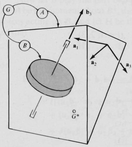
Figure 7.3.1

inertia dyadic of G , expressed in terms of K_{1},K_{2} , and K_{3} , the central principal moments of inertia of G ,is given by

\mathbf{I}_{G}=K_{1}\mathbf{a}_{1}\mathbf{a}_{1}+K_{2}\mathbf{a}_{2}\mathbf{a}_{2}+K_{3}\mathbf{a}_{3}\mathbf{a}_{3}

where {\bf a}_{1},{\bf a}_{2},{\bf a}_{3} are mutually perpendicular unit vectors fixed in \pmb{A} and parallel to central principal axes of G .The axis of symmetry of \boldsymbol{B} is parallel to a unit vector {\bf b}_{3} , and {\bf{I}}_{B} , the central inertia dyadic of \boldsymbol{B} , can be expressed as

\mathbf{I}_{B}=I(\mathbf{b}_{1}\mathbf{b}_{1}+\mathbf{b}_{2}\mathbf{b}_{2})+J\mathbf{b}_{3}\mathbf{b}_{3}

where {\bf b}_{1} and {\bf b}_{2} are unit vectors fixed in A , perpendicular to each other, and such that {\bf b}_{3}={\bf b}_{1}\times{\bf b}_{2}

When G moves in a Newtonian reference frame N in the absence of external constraints, it is convenient to work with generalized speeds u_{1},\dotsc,u_{7} defined as

\begin{array}{r l}{u_{i}\triangleq^{N}\!\mathbf{\upomega}^{A}\cdot\mathbf{a}_{i}\quad}&{{}(i=1,2,3)}\\ {u_{4}\triangleq^{A}\!\mathbf{\upomega}^{B}\cdot\mathbf{b}_{3}}\\ {u_{4+i}\triangleq^{N}\!\mathbf{\upomega}^{G^{*}}\cdot\mathbf{n}_{i}\quad}&{{}(i=1,2,3)}\end{array}

where G^{*} is the mass center of G and \mathbf{n}_{1},\,\mathbf{n}_{2},\,\mathbf{n}_{3} are mutually perpendicular unit vectors fixed in N . As generalized coordinates one can use, for example, angles q_{1},\,q_{2} , and q_{3} like those in Problem 1.1 to characterize the relative orientations of \mathbf{n}_{1},\mathbf{n}_{2},\mathbf{n}_{3} and {\bf a}_{1},{\bf a}_{2},{\bf a}_{3} ; an angle \mathbf{q_{4}} between two lines that are perpendicular to {\mathfrak b}_{3} , one line fixed in A , the other fixed in \mathbfit{B} ; and Cartesian coordinates q_{5},\,q_{6} , and \scriptstyle q_{7} of G^{*} relative to a set of axes fixed in N .Table 7.3.1 shows the relationship between {\bf a}_{1},{\bf a}_{2},{\bf a}_{3} and \mathbf{n}_{1},\mathbf{n}_{2},\mathbf{n}_{3}

Letting G play the role of s , suppose that G moves in N in the absence of external forces. Then \mathbf{R} in Eq. (1) is equal to zero and, if one takes for \mathbf{n} in Eq. (1) any one of \mathbf{n}_{1},\;\mathbf{n}_{2},\;\mathbf{n}_{3} , then Eq.(1) is satisfied because ^N d\mathbf{n}_{i}/d t=0 (i=1,2,3) .Since \mathbf{L} , the linear momentum of G in N , is given by

{\bf L}=M^{N}{\bf v}^{G^{\star}}

one can, therefore, write

{}^{N}\mathbf{v}^{G^{k}}\cdot\mathbf{n}_{i}=C_{i}\qquad(i=1,2,3)

Table 7.3.1

<html>

	a1	a2	a3
n	C2C3	-C2S3	S2
n2	SS2.C3+S3C1	-SS2S3+CC	-SC2
n3	-CS2C3+SS1	CS2S3+ C3S1	C,C2

</html>

which leads with the aid of Eqs. (15) to the three integrals

u_{4\,+\,i}=C_{i}\qquad(i=1,2,3)

In the absence of external forces, \mathbf{M} in Eq. (3) is equal to zero and, with n equal to {\mathbf{n}}_{i}\,(i=1,2,3) , Eq. (3) is satisfied. Consequently,

\mathbf{H}_{G}\cdot\mathbf{n}_{i}=C_{3\,+\,i}\qquad(i=1,2,3)

where \mathbf{H}_{G} , the central angular momentum of G in N , can be written (see Problem 6.5)

\mathbf{H}_{G}=\mathbf{I}_{G}\cdot^{N}\mathbf{\omega}\mathbf{\omega}^{A}+\mathbf{I}_{B}\cdot^{A}\mathbf{\omega}^{B}

or

\mathbf{H}_{G}\,=\,K_{1}u_{1}\mathbf{a}_{1}+K_{2}u_{2}\mathbf{a}_{2}+K_{3}u_{3}\mathbf{a}_{3}+J u_{4}\mathbf{b}_{3}

Consequently,

K_{1}u_{1}{\bf a}_{1}\cdot{\bf n}_{i}+K_{2}u_{2}{\bf a}_{2}\cdot{\bf n}_{i}+K_{3}u_{3}{\bf a}_{3}\cdot{\bf n}_{i}+J u_{4}{\bf b}_{3}\cdot{\bf n}_{i}\quad=\quad C_{3+i}\quad\quad(i=1,2,3)

Furthermore, {\bf b}_{3} can be written

\mathbf{b}_{3}=\beta_{1}\mathbf{a}_{1}+\beta_{2}\mathbf{a}_{2}+\beta_{3}\mathbf{a}_{3}

where \beta_{1},\,\beta_{2} ,and \beta_{3} are constants. Referring to Table 7.3.1, one thus arrives at the integrals

\begin{array}{r l}&{(K_{1}u_{1}+J u_{4}\beta_{1})\mathrm{c}_{2}\mathrm{c}_{3}-(K_{2}u_{2}+J u_{4}\beta_{2})\mathrm{c}_{2}\mathrm{s}_{3}+(K_{3}u_{3}+J u_{4}\beta_{3})\mathrm{s}_{2}=C_{4}}\\ &{(K_{1}u_{1}+J u_{4}\beta_{1})(\mathrm{s}_{1}\mathrm{s}_{2}\mathrm{c}_{3}+\mathrm{s}_{3}\mathrm{c}_{1})}\\ &{\qquad+\,(K_{2}u_{2}+J u_{4}\beta_{2})(-\mathrm{s}_{1}\mathrm{s}_{2}\mathrm{s}_{3}+\mathrm{c}_{3}\mathrm{c}_{1})-(K_{3}u_{3}+J u_{4}\beta_{3})\mathrm{s}_{1}\mathrm{c}_{2}=C_{5}}\\ &{(K_{1}u_{1}+J u_{4}\beta_{1})(-\mathrm{c}_{1}\mathrm{s}_{2}\mathrm{c}_{3}+\mathrm{s}_{3}\mathrm{s}_{1})}\\ &{\qquad+\,(K_{2}u_{2}+J u_{4}\beta_{2})(\mathrm{c}_{1}\mathrm{s}_{2}\mathrm{s}_{3}+\mathrm{c}_{3}\mathrm{s}_{1})+(K_{3}u_{3}+J u_{4}\beta_{3})\mathrm{c}_{1}\mathrm{c}_{2}=C_{6}}\end{array}
$$(24) (25)  

Now let $\textbf{\emph{B}}$ play the part of $s$ in connection with Eqs. (3) and (4); that is, let $\mathbf{M}$ be the moment about $B^{*}$ , the mass center of $B$ , of all contact and distance forces acting on $\pmb{B}$ , and let $\mathbf{H}$ be the central angular momentum $\mathbf{H}_{B}$ of $\pmb{B}$ in $N$ so that  

\begin{array}{r}{\mathbf{H}{B}\underset{\mathbf{\mu{2}}\mathbf{\mu_{3}}}{=}\underset{\mathbf{\mu_{2}}\mathbf{\mu_{3}}}{=},\mathbf{I}{B}\cdot\mathbf{\mu{\omega}}^{N}\mathbf{\omega}^{B}=\mathbf{I}{B}\cdot(\mathbf{\mu{\omega}}^{N}\mathbf{\omega}^{A}+\mathbf{\mu_{\omega}}^{A}\mathbf{\omega}^{B})}\end{array}

  

or  

\begin{array}{c}{{{\bf{H}}{B}\ =\ [(I({\bf{b}}{1}{\bf{b}}{1}+{\bf{b}}{2}{\bf{b}}{2})+J{\bf{b}}{3}{\bf{b}}{3}]\cdot(u{1}{\bf{a}}{1}+u{2}{\bf{a}}{2}+u{3}{\bf{a}}{3}+u{4}{\bf{b}}{3})}}\ {{(12)\quad\quad\quad\quad\quad\quad\quad\quad\quad\quad\quad\quad\quad\quad\quad\quad\quad\quad\quad\quad\quad(13)}}\ {{=\ I[(u{1}{\bf{b}}{1}\cdot{\bf{a}}{1}+u_{2}{\bf{b}}{1}\cdot{\bf{a}}{2}+u_{3}{\bf{b}}{1}\cdot{\bf{a}}{3}){\bf{b}}{1}}}\ {{\quad\quad\quad\quad\quad+\ (u{1}{\bf{b}}{2}\cdot{\bf{a}}{1}+u_{2}{\bf{b}}{2}\cdot{\bf{a}}{2}+u_{3}{\bf{b}}{2}\cdot{\bf{a}}{3}){\bf{b}}{2}]}}\ {{\quad\quad\quad\quad+\ J(u{1}{\beta}{1}+u{2}{\beta}{2}+u{3}{\beta}{3}+u{4}){\bf{b}}_{3}}}\end{array}

  

Finally, let ${\bf b}_{3}$ play the role of n in Eq. (3), and suppose that $\pmb{B}$ iscompletely free torotaterelative to $\pmb{A}$ sothat  

\mathbf{M}\cdot\mathbf{b}_{3}=0

  

Then, since  

\frac{^N d\mathbf{b}{3}}{d t}{(2.1.2)}=\mathbf{\nabla}{^0\mathrm{Q}}^{N}\mathbf{\upomega}^{A}\times\mathbf{\deltab}{3}=u_{1}\mathbf{a}{1}\times\mathbf{b}{3}+u_{2}\mathbf{a}{2}\times\mathbf{b}{3}+u_{3}\mathbf{a}{3}\times\mathbf{b}{3}

  

one can use the relationships  

\begin{array}{r l}&{\mathbf{b}{1}\cdot\mathbf{a}{1}\times\mathbf{b}{3}=\mathbf{b}{3}\times\mathbf{b}{1}\cdot\mathbf{a}{1}=\mathbf{b}{2}\cdot\mathbf{a}{1}}\ &{\mathbf{b}{2}\cdot\mathbf{a}{1}\times\mathbf{b}{3}=\mathbf{b}{3}\times\mathbf{b}{2}\cdot\mathbf{a}{1}=-\mathbf{b}{1}\cdot\mathbf{a}{1}}\end{array}

  

and so forth, to verify that  

\mathbf{H}{B}\cdot\frac{\mathbf{\nabla}^{N}d\mathbf{b}{3}}{d t}\underset{(28,30)}{=}0

  

Consequently, Eq. (3) is satisfied, and Eqs. (4) and (28) lead to the integral  

u_{1}\beta_{1}+u_{2}\beta_{2}+u_{3}\beta_{3}+u_{4}=C

  

The same integral can be found by noting that the Lagrangian $\mathscr{L}$ is here equal to the kinetic energy of $G$ in $N$ , so that (see Problem 10.8)  

\begin{array}{c}{{\mathcal{L}=\displaystyle\frac{1}{2}({K_{1}}{u_{1}}^{2}+{K_{2}}{u_{2}}^{2}+{K_{3}}{u_{3}}^{2})+J u_{4}\left(u_{1}\beta_{1}+u_{2}\beta_{2}+u_{3}\beta_{3}+\frac{u_{4}}{2}\right)}}\ {{+\displaystyle\frac{1}{2}M({u_{5}}^{2}+{u_{6}}^{2}+{u_{7}}^{2})}}\end{array}

  

and $\mathbf{q_{4}}$ is absent from $\mathscr{L}$ when $u_{1},\dotsc,u_{7}$ are expressed in terms of $q_{1},\ldots,q_{7}$ and ${\dot{q}}_{1},\dots,\ {\dot{q}}_{7}$ ; however, $\dot{q}_{4}$ appears in Eq. (35) because $u_{4}=\dot{q}_{4}$ . Consequently,  

{\frac{\partial{\mathcal{L}}}{\partial{\dot{q}}{4}}}={\frac{\partial{\mathcal{L}}}{\partial u{4}}}{(35)}=J(u{1}\beta_{1}+u_{2}\beta_{2}+u_{3}\beta_{3}+u_{4})

  

and, setting the right-hand member of this equation equal to a constant in accordance with Eq. (5), one recovers Eq. (34).  

The integrals reported in Eqs. (18) and (24) also can be obtained by using Eq. (5) in conjunction with Eq. (35), but those expressed in Eqs. (25) and (26) cannot, for $q_{2}$ and $q_{3}$ appear in $\mathcal{L}$ when $u_{1},u_{2}$ , and $\pmb{u}_{3}$ are replaced inEq.(35) with  

\begin{array}{l}{{u_{1}=\dot{q}{1}\mathrm{c}{2}\mathrm{c}{3}+\dot{q}{2}\mathrm{s}{3}}}\ {{,}}\ {{u{2}=-\dot{q}{1}\mathrm{c}{2}\mathrm{s}{3}+\dot{q}{2}\mathrm{c}{3}}}\ {{,}}\ {{u{3}=\dot{q}{1}\mathrm{s}{2}+\dot{q}_{3}}}\end{array}

  

respectively.  

# 7.4EXACT CLOSED-FORM SOLUTIONS  

Usually, it is difficult to find in closed form the exact, general solution of the equations of motion of a system S (see Sec. 7.1) because the differentiai equations governing the generalized coordinates and generalized speeds are both nonlinear and coupled. At times, some of the generalized coordinates and/or generalized speeds can be expressed as explicit, elementary functions of time, whereas the rest cannot be so expressed. Moreover, there exists no generai, systematic procedure that facilitates the search for closed-form solutions. To find them, one must take advantage of special features of theproblem under consideraticn.  

Example In Fig. 7.4.1, $s$ represents a uniform sphere of radius $r$ that rolls on the interior surface of a fixed tube $T$ of radius $R$ , the axis of $T$ being vertical Generalized speeds $u_{1},\dotsc,u_{5}$ may be introduced as  

\begin{array}{r l}{u_{i}\triangleq\mathbf{o}\cdot\mathbf{e}{i}\quad}&{{}(i=1,2,3)}\ {u{4}\triangleq\mathbf{v}\cdot\mathbf{e}{2}\quad}&{{}u{5}\triangleq\mathbf{v}\cdot\mathbf{e}_{3}}\end{array}

  

where $\mathbf{\omega}$ is the angular velocity of $S,\,\mathbf{v}$ is the velocity of the center of $s$ and $\mathbf{e}_{1},\,\mathbf{e}_{2}$ ,and ${\bf e}_{3}$ form a right-handed set of mutually perpendicular unit vectors directed as shown in Fig. 7.4.1. For generalized coordinates one can use, in part, angles $q_{1},\,q_{2}$ ，and $q_{3}$ ,like those in Problem 1.1, to characterize the orientation of unit vectors $\mathbf{s}_{1},\,\mathbf{s}_{2},\,\mathbf{s}_{3}$ fixed in S relative to the unit vectors $\mathbf{e}_{1},\mathbf{e}_{2},\mathbf{e}_{3}$ , and, for the rest, the distance $q_{4}$ and the angle $q_{5}$ shown in Fig. 7.4.1. The kinematical differential equations then are  

![](images/46b7a5e90848262887a7fc0baa9dd6676522c3faf534f9da8086b1b392dcf638.jpg)  
Figure 7.4.1  

\begin{array}{r l}&{\dot{q}{1}=u{1}+\tan q_{2}\left[\left(u_{2}-\frac{u_{5}}{R-r}\right)s_{1}-u_{3}c_{1}\right]}\ &{\dot{q}{2}=\left(u{2}-\frac{u_{5}}{R-r}\right)c_{1}+u_{3}s_{1}}\ &{\dot{q}{3}=-\sec q{2}\left[\left(u_{2}-\frac{u_{5}}{R-r}\right)s_{1}-u_{3}c_{1}\right]}\ &{\dot{q}{4}=u{4}}\ &{\dot{q}{5}=\frac{u{5}}{R-r}}\end{array}

  

The system possesses three degrees of freedom because the two nonholonomic constraint equations (see Sec. 2.13)  

u_{4}=r u_{3}

  

and  

u_{5}=-r u_{2}

  

must be satisfied in order that there be no slipping at the contact between $\boldsymbol{s}$ and $T.$ Finally, with the aid of Eqs. (6.1.1), one can write the dynamical equations  

\begin{array}{l}{\displaystyle{\dot{u}}{1}=\frac{r}{R-r},u{2},u_{3}}\ {\displaystyle{\dot{u}}{2}=0}\ {\displaystyle{\dot{u}}{3}=,-,\frac{1}{7}\bigg(\frac{2r}{R-r},u_{1}u_{2}+\frac{5g}{r}\bigg)}\end{array}

  

In principle, Eqs. (3)-(12) sufice for the determination of $q_{1},\ldots,q_{5}$ and $u_{1},\ldots,u_{5}$ as functions of the time $t$ ; but, as will now be shown, it is considerably easier to find explicit expressions for $u_{1},\ldots,u_{5},\,q_{4}$ , and $\pmb q_{5}$ than for q1, q2, and q3.  

Equation (11) has the general solution  

u_{2}=u_{2}(0)

  

where $u_{2}(0)$ denotes the value of $\pmb{u}_{2}$ at $t=0,$ Hence,  

u_{5}=-r u_{2}(0)

  

and  

{\dot{q}}{5}\mathrel{\mathop:}{(7,14)}{\frac{r u_{2}(0)}{r-R}}

  

which has the general solution  

q_{5}=\frac{r u_{2}(0)t}{r-R}+q_{5}(0)

  

Next, if $u_{2}(0)\neq0$ , then  

u_{1},=,\frac{r,-,R}{2r u_{2}(0)}\left(\frac{5g}{r}+7\dot{u}_{3}\right)

  

so that  

\dot{u}{1}\mathop{=}{(17)}\frac{7(r-R)}{2r u_{2}(0)},\ddot{u}_{3}

  

and  

\frac{7(r-R)}{2r u_{2}(0)},\ddot{u}{3},=,\frac{r}{R-r},u{2}(0)u_{3}

  

which, after $p$ has been defined as  

p\triangleq\frac{r|u_{2}(0)|\sqrt[]{\frac{2}{7}}}{R-r}

  

can be written  

\ddot{u}{3}\mathrm{+}p^{2}u{3}=0

  

The general solution of this equation is  

u_{3}=u_{3}(0)\cos p t+\left[\frac{\dot{u}_{3}(0)}{p}\right]\sin p t

  

where ${u_{3}}(0)$ and $\dot{u}_{3}(0)$ are the initial values of $u_{3}$ and $\dot{u}_{3}$ , respectively. Moreover,  

\dot{u}{3}(0),=,-\frac{1}{7}\biggl[\frac{2r}{R-r},u{1}(0)u_{2}(0),+,\frac{5g}{r}\biggr]

  

Hence,  

u_{3}\mathop{=}{(22,23)}u{3}(0)\cos p t-\frac{1}{7p}\biggl[\frac{2r}{R-r},u_{1}(0)u_{2}(0)+\frac{5g}{r}\biggr]\sin p t

  

and differentiation of this equation leads to an expression for $\dot{u}_{3}$ , with the aid of which one obtains from Eq. (17)  

u_{1}=\frac{r-R}{2r u_{2}(0)}\left{\frac{5g}{r}-7u_{3}(0)p\sin p t-\left[\frac{2r}{R-r},u_{1}(0)u_{2}(0)+\frac{5g}{r}\right]\cos p t\right}

  

As for $\pmb{u_{4}}$ , Eqs. (8) and (24) yield  

u_{4}=r u_{3}(0)\cos{p t}-\frac{r}{7p}\left[\frac{2r}{R-r},u_{1}(0)u_{2}(0)+\frac{5g}{r}\right]\sin{p t}

  

Finally, integrating Eq. (6) after replacing $\pmb{u_{4}}$ with the right-hand member of Eq. (26), one finds that  

q_{4}=\frac{r}{p}u_{3}(0)\sin{p t}+\frac{r}{7p^{2}}\left[\frac{2r}{R-r}u_{1}(0)u_{2}(0)+\frac{5g}{r}\right]\cos{p t}+q_{4}(0)

  

Equations (27), (16), (25), (13), (24), (26), and (14) provide expressions for $q_{4},q_{5},u_{1},u_{2},u_{3},u_{4}$ , and $\boldsymbol{u}_{5}$ , respectively, as explicit functions of time, and thus they furnish much physically meaningful information about the motion of S. For example, Eq. (16) reveals that $s^{*}$ moves in a plane that rotates with a constant angular speed of magnitude $r|u_{2}(0)|/(R-r)$ about the axis of $T.$ The motion of $s^{*}$ in this rotating plane is described completely by Eq. (27), which shows that $s^{*}$ performs an oscillatory vertical motion whose circular frequency, $\pmb{p}$ [see Eq. (20)], depends both on the initial value of $\pmb{u}_{2}$ and on the geometric parameter $R/r$ ，while the amplitude of the oscillations canbe adjusted to any desired value by a suitable choice of the initial values of $u_{1}$ $u_{2}$ , and $\pmb{u}_{3}$ . In particular, one can make the amplitude equal to zero—that is, one can make $s^{*}$ move on a horizontal circle —-by taking  

u_{3}(0)=0\qquad u_{1}(0)=-,\frac{5g(R-r)}{2u_{2}(0)r^{2}}

  

These results may conflict with one's intuition; one might expect the sphere to move downward, regardless of initial conditions. Indeed, this is what happens in reality. The reason for this discrepancy between predicted and actual motions is that certain physically unavoidable, dissipative effects, such as frictional resistance to rotation, have been left out of account in the analysis. Problem 13.9 deals with a more realistic approach.  

When the expressions for $u_{1},\,u_{2}$ , and $\pmb{u}_{3}$ available in Eqs. (25), (13), and (24), respectively, are substituted into Eqs. (3)-(5), it can be seen that $q_{1},\,q_{2}$ and $\boldsymbol{q}_{3}$ are governed by a set of coupled, nonlinear differential equations with time-dependent coefficients. Generally, solutions of such sets of equations can be found only by numerical integration.  

# 7.5 NUMERICAL INTEGRATION OF DIFFERENTIAL EQUATIONS OF MOTION  

When the dynamical (see Sec. 6.1) and/or kinematical (see Sec. 2.12) differential equations governing the motion of a system S cannot be solved in closed form (see Sec. 7.4), one can use a numerical integration procedure to determine for time $t\geqslant t_{0}$ the values of the dependent variables appearing in the equations, provided that the values of these variables are known for $t=t_{0},t_{0}$ being a particular value of $t$ . To this end, one can employ any one of many computer programs applicable to the solution of a set of $\nu$ first-order differential equations of the form  

\frac{d x_{i}}{d t}=f_{i}\left(x_{1},,.,.,.,,x_{\nu};,t\right);;;;;;\left(i=1,,.,.,,,\nu\right)

  

where $x_{1},\ldots,x_{\nu}$ are unknown functions of $t$ and $f_{1},\ldots,f_{v}$ are known, generally nonlinear functions of $x_{1},\ldots,x_{v}$ , and $t$  

Sometimes the differential equations of motion of a system are available precisely in the form of Eqs. (1). When this is the case, one can proceed directly to the numerical solution of the equations, taking care in programming to ensure that the evaluation of any expression occurring repeatedly in $f_{1},\ldots,f_{v}$ is performed only once. More frequently, at least the dynamical differential equations (see Sec. 6.1) are not immediately available in the form of Eqs. (1), for use of Eqs. (6.1.1) or (6.1.2) leads to equations of the form  

X{\dot{u}}=Y

  

where $\dot{\boldsymbol{u}}$ is a $p\times1$ matrix $[p=n$ when Eqs. (6.1.2) apply] having the time-derivative $\dot{u}_{r}$ of the generalized speed $\pmb{u}_{\pmb{r}}$ as the rth element $(r=1,\ldots,p),$ $X$ is a $\pmb{p}\times\pmb{p}$ matrix whose elements are functions of the generalized coordinates $q_{1},...,\,q_{n}$ and the time $t$ and $\pmb{Y}$ is a $\pmb{p}\times1$ matrix whose elements are functions of $q_{1},\ldots,q_{n},u_{1},\ldots,u_{n},$ and t. Under these circumstances, one must “uncouple” Eqs. (2), that is, one must solve these equations for $\dot{u}_{1},...,\dot{u}_{p}$ , in order to be able to use a computer program intended for the solution of Eqs. (1). When $\pmb{p}$ is sufficiently small, or when $\pmb{X}$ is sufficiently sparse, one can do this in analytical terms; otherwise, one must resort to the use of a computer routine that solves a set of linear equations numerically, calling this routine each time $\dot{u}_{1},...,\dot{u}_{p}$ are needed.  

When one undertakes the task of forming $X$ and Y, that is, of formulating dynamical differential equations, with a view toward performing a numerical simulation of a motion of a system S, one can take certain measures that save one considerable amounts of writing and that lead to highly efficient computer codes for the evaluation of $\pmb{X}$ and $\boldsymbol{Y},$ particularly when $\pmb{p}$ is large. The two guiding ideas here are that $\dot{u}_{1},...,\dot{u}_{p}$ must be kept in explicit evidence, and that repeated writing of any expression must be avoided. The introduction of auxiliary constants $k_{1},k_{2},\ldots$ , and auxiliary functions $Z_{1}$ $\mathbf{\phantom{}}_{1},\,\mathbf{\deltaZ}_{2},\,\dots$ of $q_{1},\ldots,q_{n},\;u_{1},\ldots,u_{n}$ and $t_{\mathrm{:}}$ enables one to reach both of these goals, as will be illustrated in connection with an example.  

Example Figure 7.5.1 is a schematic representation of a spacecraft equipped with a nutation damper. This system consists of a rigid body $\pmb{B}$ and a particle $\pmb{P}$ that moves in a tube $T,$ with $P$ attached to $\textbf{\emph{B}}$ by means of a light, linear spring $\boldsymbol{s}$ and a light, linear dashpot $\textbf{\emph{D}}$ . The axis of ${\cal T}$ is parallel to line $L_{1}$ one of the central principal axes of $\pmb{B}$ ; this axis is separated from $L_{1}$ by a distance $\pmb{b}$ ; and it lies in the $L_{1}L_{2}$ plane, where $L_{2}$ , like $L_{1}$ , is a central principal axis of $\pmb{B}_{\ast}$ . The force R exerted on $\pmb{P}$ by $s$ and $\pmb{D}$ is given by  

{\bf R}=-(\sigma q+\delta\dot{q}){\bf b}_{1}

  

![](images/a636f4b9626f801927938be8fae782d1f1fe62f859af47efc3e508d26f35c6dc.jpg)  
Figure 7.5.1  

where $\sigma$ and $\delta$ are constants, $q$ is the distance from $L_{2}$ to $P$ and ${\bf b}_{1}$ is a unit vector parallel to $L_{1}$  

When the spacecraft moves in a Newtonian reference frame $N$ in the absence of external forces, then $\mathbf{H}$ the central angularmomentum of the spacecraft, remains fixed in $N$ ,but $\boldsymbol{\theta}$ , the angle between $L_{1}$ and $\mathbf{H}$ varies with time. The time-history of $\boldsymbol{\theta}$ is tobedetermined.  

Once $\mathbf{H}$ is known as a function of $t$ $\theta$ can be found with the aid of the re lationship  

\theta=\cos^{-1}!\left(\mathbf{b}_{1}\cdot{\frac{\mathbf{H}}{|\mathbf{H}|}}\right)

  

Asfor $\mathbf{H}$ ,Eqs. (3.5.27), (3.5.28), and the theorem stated in Problem 6.3 lead to  

\mathbf{H}=\mathbf{I}\cdot\mathbf{\mathcal{N}}\mathbf{\Theta}^{B}+m_{B}\mathbf{p}^{C B^{\star}}\times\mathbf{\mathcal{N}}\mathbf{v}^{B^{\star}}+m_{P}\mathbf{p}^{C P}\times\mathbf{\mathcal{N}}\mathbf{v}^{P}

  

where I is the central inertia dyadic of $\pmb{B}_{\pmb{\cdot}}$ $\pmb{N}_{\mathbf{G}\mathbf{\mathfrak{d}}^{B}}$ is the angular velocity of $\pmb{B}$ in $N$ $m_{B}$ and $m_{P}$ are the masses of $\pmb{B}$ and $\pmb{P}$ , respectively, $c$ denotes the mass center of the system formed by $\pmb{B}$ and $P$ $\mathfrak{p}^{C B^{\star}}$ and $\pmb{\mathsf{p}}^{c P}.$ are, respectively, the position vectors from $c$ to $B^{*}$ , the mass center of $\pmb{B}$ , and $c$ to $\pmb{P}$ , and $\aleph_{\mathbf{v}}\mathbf{\cal{B}^{\star}}$ and $\pmb{N}_{\mathbf{v}}\pmb{P}$ are,respectively, the velociti o $B^{*}$ and $\pmb{P}$ .n $N$ Hence, we must detemine $^N{\bf\epsilon}_{\bf{\epsilon}}^{B},\,{\bf p}^{C B^{\star}},\,\bar{{\cal N}}_{\bf{v}}^{B^{\star}},\,{\bf p}^{C P}$ , and $\mathbf{\Delta}^{N}\mathbf{v}^{P}$ as functions of t. To this end, we shall introduce generalized speeds $u_{1},\dots,u_{7}$ in such a way that each of the required vectors can be expressed as a function of $u_{1},\dotsc,u_{7}$ , and $\pmb q$ ; formulate generalized inertia forces $F_{1}{}^{*},\ldots,F_{7}{}^{*}$ and generalized active forces $F_{1},\ldots,F_{7}$ ; use Eqs. (6.1.2) to write dynamical differential equations governing $u_{1},\dots,u_{7}$ ; and solve these numerically together with a kinematical differential equation that will be stated presently, thus obtaining $u_{1},\dotsc,u_{7},$ and $\pmb q$ as functions of $\pmb{t}$  

The generalized speeds to be employed are defined as  

\begin{array}{r l}{u_{i}\triangleq^{N}!\mathbf{\upomega}^{B}\cdot\mathbf{b}{i}\quad}&{(i=1,2,3)}\ {u{4}\triangleq\dot{q}}\ {u_{4+i}\triangleq^{N}!\mathbf{\upomega}^{B^{\star}}\cdot\mathbf{b}_{i}\quad}&{(i=1,2,3)}\end{array}

  

where ${\mathfrak{b}}_{2}$ and ${\mathfrak{b}}_{3}$ are unit vectors,' with ${\mathfrak{b}}_{2}$ parallel to $L_{2}$ , and ${\bf b}_{3}={\bf b}_{1}\times{\bf b}_{2}$ Equation (7) is the aforementioned kinematical differential equation, and the vectors appearing in Eq. (5) can be expressed in terms of $u_{1},\dotsc,u_{7}$ , and $\pmb q$ asfollows:  

\begin{array}{r c l}{{^{N}{\bf{0}}^{B}}}&{{=}}&{{u_{1}{\bf{b}}{1}+u{2}{\bf{b}}{2}+u{3}{\bf{b}}{3}}}\ {{}}&{{}}&{{}}\ {{{\bf{0}}^{C B^{*}}}}&{{=}}&{{-;\frac{m{P}}{m_{B}+m_{P}}(q{\bf{b}}{1}+b{\bf{b}}{2})}}\ {{}}&{{}}&{{(3.1.2);;;}}\ {{^{N}{\bf{0}}^{B^{*}}}}&{{=}}&{{u_{5}{\bf{b}}{1}+u{6}{\bf{b}}{2}+u{7}{\bf{b}}{3}}}\ {{}}&{{}}&{{}}\ {{{\bf{0}}^{C P}}}&{{=}}&{{\frac{m{B}}{m_{B}+m_{P}}(q{\bf{b}}{1}+b{\bf{b}}{2})}}\end{array}

  

and [use Eqs. (2.8.1), (2.7.1), (7), and (9)-(12)]  

{\bf\nabla}^{N}{\bf v}^{P}=(u_{5}+u_{4}-u_{3}b){\bf b}{1}+(u{6}+u_{3}q){\bf b}{2}+(u{7}+u_{1}b-u_{2}q){\bf b}_{3}

  

Reference to Eqs. (4.11.2), (4.11.3), (4.11.6), and (4.11.7) allows one to express $F_{r}^{\star}$ as  

F_{r}{}^{}={}^{N}!\mathfrak{w}_{r}{}^{B}\cdot\mathbf{T}^{}-m_{B}{}^{N}\mathfrak{v}{r}{}^{B^{}}\cdot{}^{N}!\mathfrak{a}^{B^{}}-m{P}{}^{N}\mathfrak{v}_{r}{}^{P}\cdot{}^{N}!\mathfrak{a}^{P}\qquad(r=1,\dots,7)

  

where $\mathbf{T^{*}}$ is the inertia torque for $\pmb{B}$ in $N,\,^{N}\mathbf{a}^{B^{\star}}$ and $\pmb{x}_{\pmb{\mathrm{g}}}P\$ are the accelerations of $B^{*}$ and $\pmb{P}$ n $N$ and $^N\!_{\mathbf{\Theta}_{r}}\bar{B},\,^{N}\!_{\mathbf{V}_{r}}\bar{B}^{\star}$ and $^N\mathbf{v}_{r}^{\textit{P}}(r=1,\ldots,7)$ are partial angular velocities of $\pmb{B}$ in $N$ and partial velocities of $B^{*}$ and $\pmb{P}$ in $N$ .As for $F_{r}$ , since it is presumed that the spacecraft moves in $N$ in the absence of external forces, the only forces that contribute to $F_{r}$ are the force $\pmb{\mathbb{R}}$ given by Eq. (3) and the reaction to this force, that is, a force $-\pmb{\mathrm{R}}$ applied to $\textbf{\emph{B}}$ at some point along the axis of $T,$ such as the point $Q$ shown in Fig. 7.5.1. Hence, $F_{\mathrm{,}}$ is given by  

F_{r}=^{N}!\mathbf{v}{r}!^{\footnotesize,P}\cdot\mathbf{R}+^{N}!\mathbf{v}{r}!^{\footnotesize,Q}\cdot\left(-\mathbf{R}\right)\quad\quad(r=1,\ldots,7)

  

where $^N\mathbf{v}_{r}^{\textit{Q}}(r=1,\ldots,7)$ are partial velocities of $Q$ in $N$  

Equations (14) and (15) show that the partial angular velocities of $\pmb{B}$ and the partial velocities of $B^{*},P_{:}$ and $Q$ are needed. Placing $Q$ (see Fig. 7.5.1) at a distance $\pmb{d}$ from $L_{2}$ (see Fig. 7.5.1), one can write  

^N\mathbf{v}^{Q}={^N\mathbf{v}^{B}}^{\star}+{^N\mathbf{\omega}\bullet^{,\ensuremath{N}}},(-d\ensuremath{\mathbf{b}}{1}+b\ensuremath{\mathbf{b}}{2})

  

or, in view of Eqs. (9) and (11),  

\mathbf{\nabla}^{N}\mathbf{v}^{Q}=(u_{5}-u_{3}b)\mathbf{b}{1}+(u{6}-u_{3}d)\mathbf{b}{2}+(u{7}+u_{1}b+u_{2}d)\mathbf{b}_{3}

  

and this brings one into position to record all necessary partial angular velocities and partial velocities as in Table 7.5.1, where numbers in parentheses in column headings refer to equations numbered correspondingly.  

The next item required for substitution into Eqs. (14) is the inertia torque $\mathbf{T}^{*}$ , which can be written  

\begin{array}{r l r}&{}&{{\bf T}^{*}\qquad=\mathrm{\boldmath~\Lambda~}-[{\dot{u}}{1}B{1}-u_{2},u_{3}(B_{2}-B_{3})]{\bf b}{1}}\ &{}&{\qquad\qquad\qquad\qquad\qquad\quad-\mathrm{\boldmath~\Lambda~}[{\dot{u}}{2}B_{2}-u_{3}u_{1}(B_{3}-B_{1})]{\bf b}{2}}\ &{}&{\qquad\qquad\qquad\quad-\mathrm{\boldmath~\Lambda~}[{\dot{u}}{3}B_{3}-u_{1}u_{2}(B_{1}-B_{2})]{\bf b}_{3}}\end{array}

  

where $B_{1},B_{2}$ , and $B_{3}$ are the moments of inertia of $\pmb{B}$ about lines $L_{1},L_{2}$ , and $L_{3}$ (see Fig. 7.5.1), respectively. At this point, the process of simplifying the analysis that follows can be begun through the introduction of constants $k_{1},k_{2},k_{3}$ as  

k_{1}\triangleq B_{2}-B_{3}\qquad k_{2}\triangleq B_{3}-B_{1}\qquad k_{3}\triangleq B_{1}-B_{2}

  

and three functions of $u_{1},u_{2}$ , and $\pmb{u}_{3}$ as  

Z_{1}\triangleq u_{2}u_{3}k_{1}\qquad Z_{2}\triangleq u_{3}u_{1}k_{2}\qquad Z_{3}\triangleq u_{1}u_{2}k_{3}

  

Table 7.5.1   


<html><body><table><tr><td></td><td>N∞,B (9)</td><td>Nv,B* (11)</td><td>Nv,P (13)</td><td>Nv,2 (17)</td></tr><tr><td>1</td><td>b1</td><td>0</td><td>bb3</td><td>bb3</td></tr><tr><td>2</td><td>b2</td><td>0</td><td>-qb3</td><td>db3</td></tr><tr><td>3</td><td>b3</td><td>0</td><td>-bb+qb2</td><td>-bb1 - db2</td></tr><tr><td>4</td><td>0</td><td>0</td><td>b1</td><td>0</td></tr><tr><td>5</td><td>0</td><td>b1</td><td>b1</td><td>b1</td></tr><tr><td>6</td><td>0</td><td>b2</td><td>b2</td><td>b2</td></tr><tr><td>7</td><td>0</td><td>b3</td><td>b3-</td><td>b3</td></tr></table></body></html>  

which makes it possible to replace Eq. (18) with  

{\bf T^{*}}{(18-20)}(-\dot{u}{1}B_{1}+Z_{1}){\bf b}{1}+(-\dot{u}{2}B_{2}+Z_{2}){\bf b}{2}+(-\dot{u}{3}B_{3}+Z_{3}){\bf b}_{3}

  

The reason for introducing $k_{1},\,k_{2}$ $k_{3}$ as in Eqs. (19) and then expressing $Z_{1},\ Z_{2},\ Z_{3}$ in terms of $k_{1},~k_{2},~k_{3}$ , rather than simply defining $Z_{1}$ as $u_{2}u_{3}(B_{2}-B_{3}).$ and similarly for $Z_{2}$ and $Z_{3}$ , is that $k_{1},\,k_{2}$ , and $k_{3}$ , being constants, can be evaluated once and for all, whereas $Z_{\scriptscriptstyle1},Z_{\scriptscriptstyle2}$ , and $Z_{3}$ , being functions of the dependent variables $u_{1},\,u_{2}$ , and $u_{3}$ , must be evaluated repeatedly in the course of a numerical integration. Hence, if $Z_{1}$ were defined as $u_{2}u_{3}\,(B_{2}-B_{3}),$ the subtraction of $B_{3}$ from $B_{2}$ would have to be performed repeatedly, but if $Z_{1}$ is defined as in the first of Eqs. (20), then this subtraction takes place only once.  

To form suitable expressions for $\mathbf{\Delta}\mathbf{x}_{\mathbf{a}}\mathbf{\scriptscriptstyle}B^{\bullet}$ and $\mathbf{v_{z}}P_{.}$ the two vectors in Eqs. (14) that have not yet been considered in detail, we differentiate Eqs. (11) and (13) with respect to $t$ in $N$ , obtaining [see Eqs. (2.6.2) and (2.3.1)] in the first case  

^N\mathbf{a}^{B^{\star}},=,\dot{u}{5},\mathbf{b}{1},+,\dot{u}{6},\mathbf{b}{2},+,\dot{u}{7},\mathbf{b}{3},+,^{N}\mathbf{\omega}\mathbf{\omega}^{B},\times,^{N}\mathbf{v}^{B^{\star}}

  

or, after using Eq. (9),  

\begin{array}{r l}{^{^N}\mathbf{a}^{B^{\star}}\ \underset{^{(9,11)}}{=}(\dot{u}{5}+u{2}u_{7}-u_{3}u_{6})\mathbf{b}{1}+(\dot{u}{6}+u_{3}u_{5}-u_{1}u_{7})\mathbf{b}{2}}&{}\ {\qquad+\ (\dot{u}{7}+u_{1}u_{6}-u_{2}u_{5})\mathbf{b}_{3}}&{}\end{array}

  

which we simplify by letting  

\begin{array}{r}{Z_{4}\triangleq u_{2}u_{7}-u_{3}u_{6}}\ {Z_{5}\triangleq u_{3}u_{5}-u_{1}u_{7}}\ {Z_{6}\triangleq u_{1}u_{6}-u_{2}u_{5}}\end{array}

  

whereupon we have  

{}^{\scriptscriptstyle N}{\bf a}^{\scriptscriptstyle B}{}^{\scriptscriptstyle*}=,(\dot{u}{\scriptscriptstyle5}+Z{4}){\bf b}{\scriptscriptstyle1}+(\dot{u}{\scriptscriptstyle6}+Z_{5}){\bf b}{\scriptscriptstyle2}+(\dot{u}{\scriptscriptstyle7}+Z_{6}){\bf b}_{\scriptscriptstyle3}

  

Similarly,  

\begin{array}{r l}&{^{N}\mathbf{a}^{P}=(\dot{u}{5}+\dot{u}{4}-\dot{u}{3}b)\mathbf{b}{1}+(\dot{u}{6}+\dot{u}{3}q+u_{3}\dot{q})\mathbf{b}{2}}\ &{\qquad(^{13})\qquad}\ &{\qquad+;(\dot{u}{7}+\dot{u}{1}b-\dot{u}{2}q-u_{2}\dot{q})\mathbf{b}_{3}+^{N}\mathbf{\omega}^{B}\times^{N}\mathbf{v}^{P}}\end{array}

  

and here it is advantageous to introduce Z's that not only permit one to write the last term in a simple form, but that at the same time accommodate those portions of the ${\mathfrak{b}}_{2}$ and ${\bf b}_{3}$ measurenumbersof $\pmb{N}_{\mathbf{\mathbfg}}P $ that do not involve ${\dot{u}}_{1},\dots,{\dot{u}}_{7}$ , that is, the two terms ${u}_{3}\dot{q}$ and $-u_{2}\dot{q},$ . which, incidentally, are respectively equal to $\boldsymbol{u}_{3}\,\boldsymbol{u}_{4}$ and $-u_{2}u_{4}$ , as can be seen by reference to Eq. (7). Specifically, we let [see Eqs. (13) and (9)]  

\begin{array}{r l}&{\begin{array}{r l}&{Z_{7}\triangleq u_{s}+u_{4}-u_{3}b}\ &{Z_{8}\triangleq u_{6}+u_{3}q}\ &{Z_{9}\triangleq u_{7}+u_{1}b-u_{2}q}\ &{Z_{10}\triangleq Z_{7}+u_{4}}\end{array}}\ &{\begin{array}{r l}&{Z_{11}\triangleq u_{2}Z_{9}-u_{3}Z_{8}}\ &{Z_{12}\triangleq u_{3}Z_{7}-u_{1}Z_{9}+u_{3}u_{4}=u_{3}Z_{10}-u_{1}Z_{9}}\ &{Z_{13}\triangleq u_{1}Z_{8}-u_{2}Z_{7}-u_{2}u_{4}=u_{3}Z_{8}-u_{2}Z_{10}}\end{array}}\end{array}

  

and this enables us to express $\mathbf{\tilde{s}_{z}}P$ as  

\begin{array}{r l}&{^{N}\mathbf{a}^{P}=~~(\dot{u}{5}+\dot{u}{4}-\dot{u}{3}b+Z{11})\mathbf{b}{1}}\ &{~~~~~~~~~~~+(\dot{u}{6}+\dot{u}{3}q+Z{12})\mathbf{b}{2}}\ &{~~~~~~~~~~~+(\dot{u}{7}+\dot{u}{1}b-\dot{u}{2}q+Z_{13})\mathbf{b}_{3}}\end{array}

  

Equations (14) and Table 7.5.1 now permit us to write  

\begin{array}{r l}&{F_{1}^{;\ast}=,-\dot{u}{1}B{1};+;Z_{1},-,m_{P}b(\dot{u}{7},+,\dot{u}{1}b,-,\dot{u}{2}q,+,Z{13})}\ &{}\ &{F_{2}^{;\ast}=,-,\dot{u}{2},B{2},+,Z_{2},+,m_{P}q(\dot{u}{7},+,\dot{u}{1}b,-,\dot{u}{2}q,+,Z{13})}\ &{\qquad\qquad\qquad\qquad\qquad\qquad\qquad\qquad\qquad\qquad\quad(36)}\ &{F_{3}^{;\ast}=,-\dot{u}{3}B{3},+,Z_{3},+,m_{P}b(\dot{u}{5},+,\dot{u}{4},-,\dot{u}{3}b,+,Z{11})}\ &{\qquad\qquad\qquad\qquad\quad\quad\quad\quad\quad\quad\quad\quad\quad\quad\quad\quad\quad\quad\quad\quad\quad}\ &{\qquad\qquad\quad\quad-,m_{P}q(\dot{u}{6},+,\dot{u}{3}q,+,Z_{12})}\end{array}

\begin{array}{l}{{F_{4}{}^{}=,-m_{P}(\dot{u}{5}+\dot{u}{4},-,\dot{u}{3}b+Z{11}),}}\ {{\ }}\ {{F_{5}{}^{}=,-m_{B}(\dot{u}{5},+,Z{4})-m_{P}(\dot{u}{5},+,\dot{u}{4},-,\dot{u}{3}b+Z{11}),}}\ {{\ }}\ {{F_{6}{}^{}=,-m_{B}(\dot{u}{6},+,Z{5})-m_{P}(\dot{u}{6},+,\dot{u}{3}q,+,Z_{12}),}}\ {{\ }}\ {{F_{7}{}^{}=,-m_{B}(\dot{u}{7},+,Z{6})-m_{P}(\dot{u}{7},+,\dot{u}{1}b,-,\dot{u}{2}q,+,Z{13}),}}\end{array}

  

and detailed expressions for $F_{1},...,F_{7}$ can be formed by substituting from Table 7.5.1 and Eq. (3) into Eqs. (15), with $\dot{\pmb q}$ replaced by $\pmb{u_{4}}$ [see Eq. (7)] in Eq. (3). This leads to  

\begin{array}{c}{{F_{1}=F_{2}=F_{3}=F_{5}=F_{6}=F_{7}=0}}\ {{\ \ \ \ \ \ \ \ \ \ F_{4}=-(\sigma q+\delta u_{4})}}\end{array}

  

Before using Eqs. (37)-(45) in conjunction with Eqs. (6.1.2) to write dynamical differential equations, we note that certain combinations of constants and functions appear repeatedly in Eqs. (37)-(43). Accordingly, we define $k_{4},\ldots,k_{8}$ and $Z_{14},Z_{15},Z_{16}$ as  

\begin{array}{r l}&{k_{4}\triangleq m_{P}b}\ &{k_{5}\triangleq k_{4}b}\ &{k_{6}\triangleq B_{1}+k_{5}}\ &{k_{7}\triangleq B_{3}+k_{5}}\ &{k_{8}\triangleq m_{B}+m_{P}}\end{array}

  

and  

\begin{array}{l}{{Z_{14}\triangleq m_{P}q}}\ {{Z_{15}\triangleq Z_{14}q}}\ {{Z_{16}\triangleq k_{4}q}}\end{array}

  

whereupon we find that Eqs. (6.1.2) and (37)-(53) yield  

\begin{array}{c}{{-k_{6}\dot{u}{1}+Z{16}\dot{u}{2}-k{4}\dot{u}{7}=-Z{1}+k_{4}Z_{13}}}\ {{{\displaystyle Z_{16}\dot{u}{1}-(B{2}+Z_{15})\dot{u}{2}+Z{14}\dot{u}{7}=-Z{2}-Z_{14}Z_{13}}}}\ {{{\displaystyle-(k_{7}+Z_{15})\dot{u}{3}+k{4}\dot{u}{4}+k{4}\dot{u}{5}-Z{14}\dot{u}{6}=-Z{3}-k_{4}Z_{11}+Z_{16}\dot{u}{7}+}}}\ {{{\displaystyle k{4}\dot{u}{3}-m{P}\dot{u}{4}-m{P}\dot{u}{5}=m{P}Z_{11}+\sigma q+\delta u_{4}}}}\ {{{\displaystyle k_{4}\dot{u}{3}-m{P}\dot{u}{4}-k{8}\dot{u}{5}=m{B}Z_{4}+m_{P}Z_{11}}}}\ {{{\displaystyle-Z_{14}\dot{u}{3}-k{8}\dot{u}{6}=m{B}Z_{5}+m_{P}Z_{12}}}}\ {{{\displaystyle-k_{4}\dot{u}{1}+Z{14}\dot{u}{2}-k{8}\dot{u}{7}=m{B}Z_{6}+m_{P}Z_{13}}}}\end{array}

  

and these equations have precisely the form of Eqs. (2) if the elements $X_{i j}$ and $Y_{i}\left(i,j=1,\ldots,7\right)$ of $X$ and $Y$ are taken to be (only nonzero elements are displayed)  

\begin{array}{r l}{X_{11}}&{=-k_{6}\phantom{-2}X_{12}=X_{21}\phantom{-2}\phantom{-}Z_{16}\phantom{-2}X_{17}\phantom{-2}=X_{71}\phantom{-2}\phantom{-}Y_{14}\phantom{-2}}\ {\Lambda_{22}}&{=\phantom{-}(B_{2}+Z_{16})\phantom{-2}\phantom{-}X_{27}\phantom{-2}\phantom{-}Z_{16}\phantom{-2}\phantom{-}Z_{14}}\ {\Lambda_{33}}&{=\phantom{-}(k_{7}+Z_{15})\phantom{-2}X_{34}\phantom{-2}\phantom{-}X_{35}\phantom{-2}\phantom{-}X_{43}}\ {X_{35}}&{=\phantom{-}\Lambda_{53}=k_{4}\phantom{-2}\phantom{-}X_{36}\phantom{-2}\phantom{-}X_{63}\phantom{-2}X_{63}=-Z_{14}}\ {\Lambda_{34}}&{=\phantom{-2}!!!(\xi6,!!!s8!!!/6\phantom{-2}X_{35}\phantom{-2}\phantom{-}!!!(\xi6,!!!s8!!!/6\phantom{-2}X_{36}!!!!/6\phantom{-2}X_{16}!!!!/6\phantom{-2}X_{16}!!!!/6\phantom{-2}X_{16}!!!!/6\phantom{-2}X_{16}}\ {X_{44}}&{=-m_{P}}&{X_{45}\phantom{-2}\phantom{-2}!!!(\xi7,!!!s8!!!/6\phantom{-2}X_{72}\phantom{-2}!!!!/6\phantom{-2}}\ {X_{55}}&{=-k_{8}\phantom{-2}!!!!}&{X_{66}\phantom{-2}!!!/6\phantom{-2}-k_{8}\phantom{-2}X_{77}\phantom{-2}!!!(\xi6,!!!s8!!!/6\phantom{-2}X_{8}!!!!/6\phantom{-2}X_{9}}\ {\Lambda_{35}}&{=\phantom{-2}!!!!}&{!!!}&{!!!!}&{!!!!(\xi8

  

and  

\begin{array}{r l}&{Y_{1}=-Z_{1}+k_{4}Z_{13}}\ &{\quad_{\mathrm{U}}=\sin\cal{Z}{1}}\ &{\quad{\mathrm{Y}{2}}=-Z{14}Z_{13}}\ &{\quad_{\mathrm{S}{3}}=-Z{3}-Z_{14}Z_{11}+Z_{14}Z_{12}}\ &{\quad_{\mathrm{S}{5}}=\sin\cal{Z}{11}+\sigma_{0}+\delta u_{4}}\ &{\quad_{\mathrm{Y}{4}}=\ m{\mathrm{P}}Z_{11}+m_{\mathrm{P}}Z_{11}}\ &{\quad_{\mathrm{V}{5}}=m{\mathrm{B}}Z_{4}+m_{\mathrm{P}}Z_{11}}\ &{\quad_{\mathrm{U}}=\sin\cal{Z}{3}+m{\mathrm{P}}Z_{12}}\ &{\quad_{\mathrm{V}{6}}=m{\mathrm{B}}Z_{6}+m_{\mathrm{P}}Z_{13}}\ &{\quad_{\mathrm{V}{7}}=m{\mathrm{B}}Z_{6}+m_{\mathrm{P}}Z_{13}}\end{array}

  

Since the matrix $X$ is relatively sparse, one can uncouple Eqs. (54)-(60) by hand, proceeding as follows: Solve Eqs. (54), (55), and (60) for $\dot{u}_{1},\;\dot{u}_{2}$ ， and $\dot{u}_{7}$ ; solve Eq. (59) for $\dot{u}_{6}$ ; substitute into Eq. (56); solve Eqs. (56), (57), and (58) for $\dot{u}_{3},\dot{u}_{4}$ , and $\dot{u}_{5}$ . The resulting equations together with Eq. (7) can be written in the form of Eqs. (1), with $\nu=8$ $x_{i}=u_{i}$ $(i=1,\cdot\cdot,7)$ , and $x_{8}=q$ , and a numerical integration of the equations can be performed, once the initial values of $u_{1},\dotsc,u_{7}$ , and $q$ , as well as the values of the parameters $m_{B},B_{1},B_{2},B_{3},b,m_{P},\sigma,$ and $\delta$ have been specified.  

Calculations leading to values of $\theta$ for various values of t can be performed simultaneously with the numerical integration of the differential equations of motion on the basis of the considerations that follow.  

With $B_{1},B_{2}$ , and $B_{3}$ as defined, $\mathbf{I}\cdot^{N}\mathbf{\omega}\mathbf{\sigma}^{B}$ is given by  

\mathbf{I}\cdot^{\aleph}!\mathbf{\dot{o}}^{B}=B_{1}u_{1}\mathbf{b}{1}+B{2}u_{2},\mathbf{b}{2}+B{3}u_{3},\mathbf{b}_{3}

  

and substitution from this equation and Eqs. (10)-(13) into Eq. (5) yields  

\mathbf{H}=H_{1}\mathbf{b}{1}+H{2}\mathbf{b}{2}+H{3}\mathbf{b}_{3}

  

where  

\begin{array}{r l}&{H_{1}\triangleq B_{1}u_{1}+b Z_{17}}\ &{H_{2}\triangleq B_{2}u_{2}-q Z_{17}}\ &{H_{3}\triangleq B_{3}u_{3}+k_{9}[u_{3}q^{2}-b(u_{4}-u_{3}b)]}\end{array}

  

with  

k_{9}\triangleq\frac{m_{B}m_{P}}{k_{8}}\qquad Z_{17}\triangleq k_{9}(Z_{9}-u_{7})

  

Consequently,  

\centering\theta=\cos^{-1}{\frac{H_{1}}{({H_{1}}^{2}+{H_{2}}^{2}+{H_{3}}^{2})^{1/2}}}

  

The quantity $({H_{1}}^{2}+{H_{2}}^{2}+{H_{3}}^{2})^{1/2}$ is of interest not only in this connection, but also because it must remain constant throughout the motion of the spacecraft[set $\mathbf{M}=0$ in Eq. (7.3.9) and note Eq. (74)], and its evaluation at various instants during a numerical integration can thus serve as a check on the validity of the integration results.  

Turning to some concrete examples in order to illustrate the uses of numerical simulations of motions, we let $B$ be a uniform rectangular parallelepiped having edges of lengths $1.2{\:}{\bf m},1.225{\:}{\bf m}$ and $1.3\,\mathbf{m}$ , these edges being respectively parallel to $L_{1},L_{2},L_{3}$ , and assume that $B$ has a mass density of $2760\ \mathrm{kg/m}^{3}$ (the mass density of aluminum), so that $m_{B}=2760\times\,1.2\,\times\,1.225\,\times\,1.3=$ $5274.4~\mathrm{\bf~kg}.$ 、while $B_{1}=5274.4\,\times\,(1.225^{2}\,+\,1.3^{2})/12=1402.4\,\mathrm{\kg\m^{2}},$ $B_{2}=$ $5274.4\,\times\,(1.3^{2}+1.2^{2})/12=1375.7\,\mathrm{kg}\,\mathrm{m}^{2}$ $B_{3}=5274.4\times(1.2^{2}+1.225^{2})/12$ $=1292.5\;\mathbf{kg}/\mathbf{m}^{2}$ . We take $b=1.0\:\mathrm{m}$ and, after defining $\mu$ as  

\mu\triangleq{\frac{m_{P}}{m_{B}}}

  

set $m_{P}=52.744\,\mathrm{kg},$ so that $\mu=0.01$ .As for $\sigma$ and $\delta$ we choose these such that the oscillator formed by $P,\,S$ , and $_{D}$ has a circular natural frequency (see Sec. 7.10) of 1 rad/s and is critically damped (see Problem 14.9), that is, $\sigma=52.744\;\mathrm{N/m},$ and $\delta=105.49~\mathrm{Ns/m}$  

To explore what happens if the spacecraft is subjected to a small disturbance while it is performing a simple spinning motion, we begin by noting that, for all $t$ prior to the disturbance,  

{\bf\dot{\Phi}}^{N}{\bf\Phi}{\bf{C}\bf{0}}^{B}=\Omega{\bf{b}}{1}

  

where $\pmb{\Omega}$ is a constant, called the nominal spin rate. The velocity of $C$ ,the mass center of the spacecraft, is given by  

\mathbf{\nabla}^{N}\mathbf{v}^{C}=0

  

and $P$ remains on line $L_{2}$ , so that  

q=0

  

From Eqs. (9) and (81), it then follows that  

u_{1}=\Omega\qquad u_{2}=u_{3}=0

  

and Eqs. (7) and (83) imply that  

u_{4}=0

  

Furthermore,  

\begin{array}{r l}{\displaystyle^{N}\mathbf{v}^{B^{\star}}}&{=\quad_{N}^{\star}\mathbf{v}{\mathbf{v}}^{C}+,^{N}\mathbf{\Sigma}{\mathbf{0}}^{\mathbf{0}}\times,\mathbf{p}^{C B^{\star}}}\ {\displaystyle(2\cdot7.1)}&{}\ {\displaystyle\qquad=}&{,(\mathbf{\Sigma}{\mathbf{0}^{\star}}+\Omega\mathbf{b}{1}\times\left(-,\frac{m_{P}}{m_{B}+m_{P}},b\mathbf{b}{2}\right)}\ {\displaystyle(\mathbf{\Sigma}{\mathbf{0}^{\star}}}&{=\left.-\Omega,\frac{b\mu}{1+\mu},\mathbf{b}{3}=-\Omega,\frac{b}{101},\mathbf{b}{3}\right.}\end{array}

  

so that, considering Eq. (11), we conclude that, for all $t$ prior to a disturbance,  

u_{5}=u_{6}=0

  

and  

u_{7}=-\frac{\Omega b}{101}

  

Equations (84), (85), (87), (88), and (83) furnish a precise characterization of the undisturbed motion, and it may be verified with the aid of Eqs. (20), (24)-(26), (29)-(35), and (51)- (53) that the equations of motion, that is, Eqs. (7) and (54)-(60) are, in fact, satisfied when $u_{1},\dotsc,u_{7}$ ,and $q$ aregivenby Eqs. (84), (85), (87), (88), and (83), which means that the postulated motion is physically possible. Equations (75)-(79) show that $\theta=0$ during this motion.  

To study motions that ensue subsequent to a slight disturbance of the motion under consideration, we perform numerical simulations after assigning the following initial values to $u_{1},\dotsc,u_{7}$ ,and $q$  

\begin{array}{l}{{u_{1}(0)=\Omega+\varepsilon_{1}}}\ {{\displaystyle u_{i}(0)=\varepsilon_{i}\qquad(i=2,\ldots,6)}}\ {{\displaystyle u_{7}(0)=,-,\frac{\Omega b}{101}+\varepsilon_{7}}}\end{array}

  

and  

q(0)=\eta

  

where $\varepsilon_{1},\ldots,\varepsilon_{7}$ ，and $\eta$ are constants called  initial perturbations. With $\Omega=1.0\;\mathrm{rad/s}$ $\varepsilon_{1}=0,~\varepsilon_{2}=0.1~\mathrm{rad/s},$ $\varepsilon_{3}=\cdot\cdot\cdot=\varepsilon_{7}=\eta=0$ this leads to the $\theta$ versus $t$ plot displayed in Fig. 7.5.2, which shows that the associated disturbance causes $\theta$ to have a nonzero initial value and to perform oscillations with decaying amplitudes. When the value of $\varepsilon_{2}$ is reduced to $0.05\,\mathrm{\rad/s}$ one-half of its former value, one might expect the amplitudes of the oscillations to be smaller than they were previously, and indeed they are, as can be seen in Fig. 7.5.3.  

To see that $P,s,$ and $_{D}$ do, in fact, serve as a nutation damper, one can perform a simulation differing in only one respect from the one that led to Fig. 7.5.2, namely, in that it applies when $m_{P}$ is equal to zero. The resulting $\theta$ versus $t$ curve, shown in Fig. 7.5.4, reveals that oscillations in $\theta$ fail to decay when $m_{P}=0.$ In other words, there is no damping under these circumstances.  

![](images/decc904063ef5da167ee2fb8411b8afecfcab54a9d2c58d2d50a1e3eb89c82cd.jpg)  

Figure 7.5.2  

![](images/0c4fde26454bd7ff0816a49ce5c8a686fab0f91b16c3d662964ada3f834654fd.jpg)  

Figure 7.5.3  

![](images/0b794ecc878f0ec5b4b97f9d2217bf418c6f36ab24bf87be1ded3db31098643d.jpg)  

Figure 7.5.4  

216 EXTRACTION OF INFORMATION FROM EQUATIONS OF MOTION 7.5  

![](images/08c4a8e9f7d734ddaf79d12993012ecadce7b069f7c37eef77f0d4f52cc58033.jpg)  

Figure 7.5.5  

![](images/1a2ecdb457a713c844d75b8608deef98dc741cf4698264c7113286d31abb58e2.jpg)  

To see that $P,s,$ and $\boldsymbol{D}$ can act as a nutation generator, rather than as a nutation damper, one can change the dimensions of the edges of $B$ parallel to $L_{1},\,L_{2}$ , and $L_{3}$ to $0.5\,\textrm{m}$ $1.2\,\textrm{m}$ , and $3.185\,\textrm{m}$ ,respectively, and set $\sigma=$ $0.52744~\mathrm{N/m}$ , so that the volume, and hence the mass, of $B$ remains unchanged, but $\sigma$ is reduced to $\frac{1}{100}$ of its former value. Letting all other quantities have the values -used in connection with Fig. 7.5.2, one then obtains Fig. 7.5.5, which portrays highly unstable attitude behavior. Moreover, a simulation differing from the one used to generate Fig. 7.5.5 only in that it applies when $m_{P}$ is equal to zero gives rise to Fig. 7.5.6, which leads to the conclusion that $P,S;$ and $\pmb{D}$ are responsible for the unstable motion depicted in Fig. 7.5.5.  

As a check on the validity of the computations underlying Figs. 7.5.2- 7.5.6, the quantity $|\mathbf{H}|\triangleq({H_{1}}^{2}+{H_{2}}^{2}+{H_{3}}^{2})^{1/2}$ [see Eq. (74)] was evaluated throughout each of the simulations used to produce these figures. In every case, $|\mathbf{H}|$ was found to remain constant to at least six significant figures.  

The preceding results are intended to underscore the fact that simulations of motions can provide valuable physical insights. The extent to which they do so depends heavily on the analyst's ingenuity in choosing parameter values and initial conditions.  

# 7.6 DETERMINATION OF CONSTRAINT FORCES AND CONSTRAINT TORQUES  

Forces and torques that make no contributions to generalized active forces are called constraint forces and constraint torques, respectively. To determine these, one uses one or more dynamical equations in which constraint force and/or constraint torque measure numbers of interest come into evidence (see Sec. 6.3), substituting into such equations values of the generalized coordinates and generalized speeds obtained by solving the kinematical and dynamical differential equations governing the motion under consideration.  

Example Figure 7.6.1 shows a linkage formed by uniform bars $A,\,B$ , and $C$ each of length $_{2L}$ , having masses $m_{A},\,m_{B}$ , and $m_{C}$ , respectively. Supported by horizontal pins at $P$ and S, the linkage is free to move in a vertical plane, and such motions are governed by the differential equations  

![](images/b8c3220e90f1c8615f9d1e68daa293f5de51e230f386e55583d8e89455160e85.jpg)  
Figure 7.6.1  

\begin{array}{l}{{\dot{q}}{1}=u{1}}\ {{\dot{u}}{1}=-p^{2}\mathbf{s}{1}}\end{array}

  

where $q_{1}$ is the radian measure of an angle as indicated in Fig. 7.6.1, $u_{1}$ is a generalized speed defined such that Eq. (1) is satisfied, $\mathbf{s}_{1}\triangleq$ sin $\pmb q_{1}$ and $\pmb{p}$ is a constant defined as  

p\triangleq\left[\frac{3g(m_{A}+m_{B}+2m_{C})}{4L(m_{A}+m_{B}+3m_{C})}\right]^{1/2}

  

The set of forces exerted on $A$ by the pin at $\pmb{P}$ can be replaced with a couple whose torque is perpendicular to $\mathfrak{n}_{3}$ (see Fig. 7.6.2 for $\begin{array}{r}{\overline{{\bf\nabla}}\equiv\!\!\begin{array}{r}{{\bf\nabla}\;}\\ {{\bf\nabla}\;}\end{array}$ ), together with a force $R_{1}\mathbf{n}_{1}+R_{2}\mathbf{n}_{2}+R_{3}\mathbf{n}_{3}$ applied to $A$ at $P.\;R_{1}$ is to be determined for $t=9\,\mathfrak{s}$ and $t=10\,\mathbf{s}.$ with $m_{A}=1\,\mathbf{k}\mathbf{g}$ $m_{B}=2\,\mathbf{k}\mathbf{g}$ $m_{c}=3\,{\bf k g},$ $L=1\;\mathbf{m}$ and $q_{1}(0)=30^{\circ}$ $u_{1}(0)=0$  

![](images/789a9f41ea28008d4e8075f0a42764f90bdf9da42602950d54fead62a111a92c.jpg)  
Figure 7.6.2  

To bring $R_{1}$ (but not $R_{2},\,R_{3}$ , or the torque of the couple exerted on $A$ by the pin) into evidence, one can imagine that $P$ is attached to a slider that is free to move in a horizontal slot, as indicated in Fig. 7.6.2, and one can introduce a generalized speed $u_{2}$ such that the velocity of $P$ is given by (see Fig. 7.6.2 for $\mathfrak{n}_{1}$  

\mathbf{v}^{P}=u_{2},\mathbf{n}_{1}

  

The angular velocities of $A,\,B$ , and $C$ then are given by  

\mathbf{\omega}\mathbf{\omega}\mathbf{\omega}\mathbf{\omega}\mathbf{\omega}\mathbf{\omega}\mathbf{\omega}\mathbf{\omega}\mathbf{\omega}\mathbf{\omega}\mathbf{\omega}\mathbf{\omega}

  

and  

\mathbf{\omega\omega^{B}}=\beta\mathbf{n}{3}\qquad\mathbf{\omega0}^{C}=\gamma\mathbf{n}{3}

  

where $\beta$ and $\gamma$ are functions of $\boldsymbol{q}_{1},\,\boldsymbol{u}_{1}$ . and $u_{2}$ , which functions are found by setting $\mathbf{v}^{s}$ , the velocity of point $s$ , equal to zero after expressing $\mathbf{v}^{s}$ as  

\mathbf{v^{s}}\ \mathop{=}\ \mathbf{v^{P}}+\mathbf{\omega^{4}}\times(-2L\mathbf{e}{2})+\mathbf{\omega^{\mathcal{C}}}\times(2L\mathbf{n}{1})+\mathbf{\omega^{8}}\times(2L\mathbf{e}_{2})

  

Thus (see Fig. 7.6.2 for the unit vectors $\mathbf{e}_{1}$ and $\mathbf{e}_{2}$ ) one obtains  

0=u_{2}\mathbf{n}{1}+2L u{1}\mathbf{e}{1}+2L;\mathbf{n}{2}-2L\beta\mathbf{e}_{1}

  

and dot-multiplications of Eq. (8) with $\mathfrak{n}_{1}$ and $\mathbf{e}_{2}$ lead to  

\beta=u_{1}+\frac{u_{2}}{2L\mathsf{c}_{1}}

  

and  

\gamma=\frac{u_{2},\mathrm{s}{1}}{2L,\mathrm{c}{1}}

  

respectively, where $\mathfrak{c}_{1}\triangleq$ cOS $q_{1}$ . Consequently,  

\mathbf{\omega}\mathbf{\omega}{\omega{}}^{B}=\left(u_{1}+\frac{u_{2}}{2L\mathbf{c}{1}}\right)\mathbf{n}{3}

  

and  

\mathbf{\omega}\mathbf{\omega}\mathbf{\omega}^{\mathrm{C}}\underset{(6,10)}{=}\frac{u_{2},\mathbf{s}{1}}{2L\mathbf{c}{1}},\mathbf{n}_{3}

  

Furthermore, the velocities of $A^{*},B^{*}$ and $C^{*}$ , the mass centers of $A,B.$ and $C$ , respectively, are  

{\begin{array}{r l}&{{\mathbf{v}}^{4^{}}={\mathbf{v}}^{P}+{\mathbf{\Phi}}\mathbf{{\Phi}}\mathbf{{\Phi}}\times\left(-L{\mathbf{e}}{2}\right)=u{2}{\mathbf{n}}{1}+L u{1}{\mathbf{e}}{1}}\ &{{\mathbf{\Phi}}\quad={\mathbf{\Phi}}\mathbf{{v}}^{P}\times\left(-L{\mathbf{e}}{2}\right)=\left(L u_{1}+{\frac{u_{2}}{2\mathbf{c}{1}}}\right){\mathbf{e}}{1}}\ &{{\mathbf{v}}^{C^{}}={\mathbf{v}}^{Q}+{\mathbf{\Phi}}\mathbf{{\Phi}}\mathbf{{\Phi}}\times\left(L{\mathbf{n}}{1}\right)=2L u{1}{\mathbf{e}}{1}+\left({\mathbf{n}}{1}+{\frac{s_{1}}{2\mathbf{c}{1}}}{\mathbf{n}}{2}\right)u_{2}}\end{array}}

  

and with the aid of Eqs. (5), (11), (12), (13)-(15), and (4), one can formulate the partial angular velocities of $A,B,$ and $C$ and the partial velocities of $A^{*}$ $B^{*},C^{*}$ ,and $P$ associated with $u_{2}$ as  

\begin{array}{r l r l}&{\mathbf{\Phi{o_{2}}}^{A};=;0\quad}&&{\mathbf{\Phi{o_{2}}}^{B}=\frac{\mathbf{n_{3}}}{(11)}\quad}&&{\mathbf{\Phi{o_{2}}}^{C};=;\frac{\mathbf{s_{1}}\mathbf{n_{3}}}{(12)}\quad}\ &{;}&&{;}\ &{\mathbf{v_{2}}^{A^{\star}};=;\mathbf{n_{1}}\quad}&&{\mathbf{v_{2}}^{B^{\star}};=;\frac{\mathbf{e_{1}}}{(14)}\quad}&&{\mathbf{v_{2}}^{C^{\star}};=;\mathbf{n_{1}},+,\frac{\mathbf{s_{1}}\mathbf{n_{2}}}{2\mathbf{c_{1}}}\quad}\end{array}

  

and  

{\mathbf{v}{2}}^{P}=\mathbf{n}{1}

  

With $u_{2}=0$ (because this corresponds to the motion of interest), the inertia forces for $A,B.$ and $c$ are [see Eq. (4.11.3)]  

\begin{array}{r l}&{\mathbf{R}{{A}}^{\phantom{\dagger}}*=,-m{{A}}\mathbf{a}^{{A}^{\star}}=,-m_{{A}}L(\Dot{u}{1}\mathbf{e}{1}+,{u_{1}}^{2}\mathbf{e}{2})}\ &{\mathbf{R}{{B}}^{\phantom{\dagger}}*=,-m_{{B}}\mathbf{a}^{{B}^{\star}}=,-m_{{B}}L(\Dot{u}{1}\mathbf{e}{1}+,{u_{1}}^{2}\mathbf{e}_{2})}\end{array}

  

and  

{\bf R}{C}{}^{*}=,-m{C}{\bf a}^{C^{\star}}=,-2m_{C}L(\dot{u}{1}{\bf e}{1}+{u_{1}}^{2}{\bf e}_{2})

  

respectively, while the inertia torques for $A,\;B,$ and $c$ can be written [see Eq. (4.11.10)]  

\begin{array}{l}{{{\bf T}{A}{}^{*}=\mathrm{-}\frac{m{A}L^{2}}{3},\dot{u}{1}{\bf n}{3}}}\ {{{\bf T}{B}{}^{*}=\mathrm{-}\frac{m{B}L^{2}}{3},\dot{u}{1}{\bf n}{3}}}\end{array}

  

and  

{{\mathbf{T}}_{c}}{}^{\ast}=0

  

Hence, the generalized inertia force ${{F}_{2}}^{*}$ , formed as [see Eq. (4.11.7)]  

\begin{array}{r l}&{F_{2}^{\mathrm{\tiny~}}=\mathbf{\omega_{0}}^{A}\cdot\mathbf{T}_{A}^{\mathrm{\tiny~}}+\mathbf{\omega_{0}}^{A^{\star}}\cdot\mathbf{R}{A}^{\mathrm{\tiny~*}}+\mathbf{\omega{2}}^{B}\cdot\mathbf{T}{B}^{\mathrm{\tiny~*}}}\ &{\qquad\qquad+\mathbf{\omega{0}}^{B^{\star}}\cdot\mathbf{R}{B}^{\mathrm{\tiny~*}}+\mathbf{\omega{2}}^{C}\cdot\mathbf{T}{C}^{\mathrm{\tiny~*}}+\mathbf{\omega{2}}^{C^{\star}}\cdot\mathbf{R}_{C}^{\mathrm{\tiny~*}}}\end{array}

  

is given by  

\begin{array}{c}{{\displaystyle{\bf\Pi}^{*};=;;;0;-m_{A}L(\dot{u}{1}{\bf c}{1;;;(1;;-;;}u_{1}{\bf\overline{{{\bf\Pi}}}}{(1}{\bf\overline{{{\bf\Pi}}}}{s_{1}})-\frac{m_{B}L}{6{\bf c}{1}},\dot{u}{1}-\frac{m_{B}L}{2{\bf c}{1}},\dot{u}{1}}}\ {{\displaystyle{\bf\Pi}(16.23)\qquad;;(17,20)}}\ {{\displaystyle{\bf\qquad\qquad\qquad\qquad\qquad}}}\ {{\displaystyle{\bf\qquad\qquad+;;;0;;;-m_{C}L\left[\dot{u}{1}\left({\bf c}{1}+\frac{1}{{\bf c}{1}}\right)-u{1}{\bf\bar{{\bf\Pi}}}{s{1}}\right]}}\ {{\displaystyle{\bf\qquad\qquad\qquad\qquad\qquad\qquad\qquad\qquad\quad(17,21)}}}\ {{\displaystyle{=;L(m_{A}+m_{C})s_{1}u_{1}{\bf\Sigma}^{2}-L\left{m_{A}{\bf c}{1}+\frac{1}{{\bf c}{1}}\left[\frac{2}{3}m_{B}+(1+{\bf c}{1}{\bf\bar{\bf\Pi}}{0})m_{C}\right]\right}\dot{u}_{1}}}}\end{array}

  

and the generalized active force $F_{2}$ , expressed as [see Eqs. (4.6.1) and (4.8.2)] $F_{2}={\bf v_{2}}^{P}\cdot(R_{1}{\bf n}_{1}+R_{2}{\bf n}_{2}+R_{3}{\bf n}_{3})-g{\bf n_{2}}\cdot(m_{A}{\bf v_{2}}^{A^{*}}+m_{B}{\bf v_{2}}^{B^{*}}+m_{C}{\bf v_{2}}^{C^{*}})$ (27) is given by  

F_{2},=,{R_{1},-,g(m_{B},+,m_{C}),{\frac{s_{1}}{2\mathrm{c}_{1}}}}

  

Solved for $R_{1}$ , the dynamical equation obtained by substituting from Eqs. (26) and (28) into  

F_{2}+F_{2}{}^{*}\quad=\quad0

  

yields with the aid of Eq. (2)  

\begin{array}{l}{{\displaystyle R_{1}=g(m_{B}+m_{C})\frac{s_{1}}{2\mathrm{c}{1}}-L(m{A}+m_{C}){s_{1}}{u_{1}}^{2}}}\ {{\displaystyle\qquad-L\left{m_{A}\mathrm{c}{1}+\frac{1}{\mathrm{c}{1}}\left[\frac{2}{3}m_{B}+(1+\mathrm{c}{1}{}^{2})m{C}\right]\right}p^{2}\mathrm{s}_{1}}}\end{array}

  

In Table 7.6.1, values are recorded for $q_{1}$ and $u_{1}$ as found by solving Eqs. (1) and (2) numerically with $m_{A},\,m_{B},\,m_{C},\,L,\,q_{1}(0)$ and $u_{1}(0)$ as given. Using the tabulated values corresponding to $t=9\,s,$ , one finds that  

\begin{array}{r l r}{\mathbf{s}{1}=,-0.1841}&{{}}&{\mathbf{c}{1}=0.9829}\end{array}

  

and  

\begin{array}{r}{{R_{1},=,9.81(5)\frac{(-0.1841)}{2(0.9829)}-(4)(-0.1841)(-1.1358)^{2}}}\ {{-,\bigg{0.9829+\frac{1}{0.9829}\bigg[\frac{4}{3}+(1+0.9661)3\bigg]\bigg}(5.}}\end{array}

  

Table 7.6.1   


<html><body><table><tr><td>t(s)</td><td>q1 (deg)</td><td>u (rad/s)</td></tr><tr><td>0</td><td>30.000</td><td>0.0000</td></tr><tr><td>1</td><td>-20.250</td><td>-0.89243</td></tr><tr><td>2</td><td>-2.8515</td><td>1.2103</td></tr><tr><td>3</td><td>24.051</td><td>-0.72140</td></tr><tr><td>4</td><td>-29.470</td><td>0.22499</td></tr><tr><td>5</td><td>15.716</td><td>1.0325</td></tr><tr><td>6</td><td>8.4490</td><td>- 1.1657</td></tr><tr><td>7</td><td>-26.989</td><td>0.52598</td></tr><tr><td>8</td><td>27.898</td><td>0.44270</td></tr><tr><td>9</td><td>-10.608</td><td>-1.1358</td></tr><tr><td>10</td><td>-13.736</td><td>1.0784</td></tr></table></body></html>  

Similarly, for $t=10~\mathbf{s},$ Eq. (30) and the last row of Table 7.6.1 yield $R_{1}=$ $6.046~\mathrm{N}.$ . Of course, the calculation of $\pmb{R}_{1}$ in accordance with Eq. (30) can be incorporated in the computer program used to solve Eqs. (1) and (2).  

# 7.7 REAL SOLUTIONS OF A SET OF NONLINEAR, NONDIFFERENTIAL EQUATIONS  

The need to find real solutions of a set of nonlinear, nondifferential equations can arise in connection with systems at rest in a Newtonian reference frame, steady motions, motions resembling states of rest, and various other problems of mechanics, as well as other areas of applied mathematics. For instance, referring to the example in Sec. 6.5, one may wish to find a value of the steering angle $\mathbf{q_{4}}$ such that the system S remains at rest when $M,R,a,b,L,T$ and $\boldsymbol{q}_{5}$ have preassigned values. To do so, one must solve Eq. (6.5.31), which one can do easily, despite the fact that the equation is nonlinear in $q_{4}$ , for Eq. (6.5.31) leads directly to  

q_{4}=\tan^{-1}!\left[\frac{T-M g R,\sin,\theta,\sin,q_{5}}{T b/L-(M g R a/L),\sin,\theta,\cos,q_{5}}\right]

  

Frequently, however, finding such solutions is not so straightforward. Consider, for example, the steady motion problem treated in the example in Sec. 6.6, and suppose that $\theta$ is to be determined for given values of $R\Omega^{2}/g$ and $h/R$ . Since Eq. (6.6.17) cannot be solved readily for $\theta$ as a function of $R\Omega^{2}/g$ and $h/R$ , one might resort to a numerical trial-and-error procedure consisting of evaluating the lefthand member of Eq. (6.6.17) for various values of $\theta$ until one has found a value that satisfies Eq. (6.6.17) to an acceptable degree of accuracy. But trial-and-error procedures become ineffective when employed for the solution of a set of nonlinear equations, as in the example in Sec. 6.7. Here, to determine $q_{1}$ and $q_{2}$ when $L\Omega^{2}/g$ is given, one must solve Eqs. (6.7.21) and (6.7.22) simultaneously, and one can do this by employing the procedure now to be described.  

Themost general set of $n$ simultaneous equations in $n$ unknowns $x_{1},\ldots,x_{n}$ canbewritten  

f_{i}(x_{1},\ldots,x_{n})=0\qquad(i=1,\ldots,n)

  

Let $y_{1}(\tau),\ldots,y_{n}(\tau)$ be a set of $\pmb{n}$ functions of a variable $\boldsymbol{\tau}$ with $0\leq\tau\leq1$ ; take  

y_{i}(0)=k_{i}\qquad(i=1,\ldots,n)

  

where $k_{i}$ , a constant, is selected arbitrarily; and require that $y_{1}(\tau),\ldots,y_{n}(\tau)$ satisfy theequations  

f_{i}(y_{1},\dots,y_{n})=f_{i}(k_{1},\dots,k_{n})(1-\tau)\qquad(i=1,\dots,n)

  

Then, as the right-hand sides of Eqs. (4) vanish at $\tau=1$ , the functions $y_{1}(\tau),\ldots,y_{n}(\tau)$ satisfy, at $\tau=1$ , precisely the same equations as do $x_{1},\ldots,x_{n}$ [see Eqs. (2)]. Now, $y_{1}(1),\ldots,\;y_{n}(1),$ and, hence, $x_{1},\ldots,\,x_{n}$ , may be found as follows: Differentiate Eqs. (4) with respect to $\boldsymbol{\uptau}$ , thus obtaining the set of first-order differential equations  

\left.{\begin{array}{l}{\displaystyle{\frac{\partial f_{1}}{\partial y_{1}}}{\frac{d y_{1}}{d\tau}}+\cdots+{\frac{\partial f_{1}}{\partial y_{n}}}{\frac{d y_{n}}{d\tau}}=-\ f_{1}(k_{1},\ldots,k_{n})}\ {\vdots}\ {\displaystyle{\frac{\partial f_{n}}{\partial y_{1}}}{\frac{d y_{1}}{d\tau}}+\cdots+{\frac{\partial f_{n}}{\partial y_{n}}}{\frac{d y_{n}}{d\tau}}=-f_{n}(k_{1},\ldots,k_{n})}\end{array}}\right}

  

and perform a numerical integration of these equations (see Sec. 7.5), using Eqs. (3) as initial conditions and terminating the integration at $\tau=1$  

As was stated previously, $k_{1},\ldots,k_{n}$ may be assigned any values whatsoever. However, it can occur that, for certain choices of $k_{1},\ldots,k_{n}$ , some of $y_{1},\dotsc,y_{n}$ do not possess real values for some values of $\boldsymbol{\uptau}$ in the interval $0\leq\tau\leq1$ , in which event the numerical integration of the differential equations cannot be carried to completion. When this happens, one simply changes one or more of $k_{1},\ldots,k_{n}$ In general, results are obtained most expeditiously when $k_{1},\ldots,k_{n}$ are good approximations to $x_{1},\ldots,x_{n}$ , respectively. Fortunately, in connection with physical problems, one often can make good guesses regarding $x_{1},\ldots,x_{n}$ , and hence assign suitable values to $k_{1},\ldots,k_{n}$ . Finally, it is worth noting that two or more distinct sets of values of $k_{1},\ldots,k_{n}$ can lead to the same values of $x_{1},\ldots,x_{n}$  

Example If $q_{1},q_{2}$ , and $q_{3}/L$ in Problem 12.6 are replaced with $x_{1},x_{2}$ , and $\pmb{x_{3}}$ ， respectively, then $x_{1},\,x_{2}$ , and $x_{3}$ are governed by equations having the form of Eqs. (2) with $n=3$ and  

\begin{array}{l}{{f_{1}\triangleq(1-s_{1})^{2}+\left(\frac{3}{2}-s_{2}\right)^{2}+(\mathrm{c}{1}-\mathrm{c}{2})^{2}-\left(x_{3}+\frac{1}{4}\right)^{2}}}\ {{,}}\ {{f_{2}\triangleq\left(x_{3}+\frac{1}{4}\right)!s_{1}+2x_{3}(\mathrm{c}{2}\mathrm{s}{1}-\mathrm{c}{1})}}\ {{,}}\ {{f{3}\triangleq\left(x_{3}+\frac{1}{4}\right)!s_{2}+2x_{3}\left(\mathrm{c}{1}\mathrm{s}{2}-\frac{3}{2},\mathrm{c}_{2}\right)}}\end{array}

  

where ${\bf s}_{i}$ and ${\bf{c}}_{i}$ now stand for sin $x_{i}$ and cos $x_{i}$ , respectively $(i=1,2)$ . The equations corresponding to Eqs. (5) are  

\begin{array}{r l}{2(s,c_{1}-c_{1})\frac{d}{d t}+2\biggl(c_{1}s_{2}-\frac{3}{2}c_{1}\biggr)\frac{d\tau_{1}}{d t}-2\biggl(r_{1}+\frac{1}{4}\biggr)\frac{d\tau_{1}}{d t}}&{}\ {=-\biggl[(1-\sin k_{1})^{2}+\biggl(\frac{3}{2}-\sin k_{2}\biggr)^{2}}&{}\ {+(\cos k_{1}-\cos k_{2})^{2}-\biggl(k_{1}+\frac{1}{4}\biggr)^{2}\biggr]}&{}\ {\biggl[\biggl(r_{1}+\frac{1}{4}\biggr)c_{1}+2y_{1}(c_{1}c_{1}+s_{1})\biggr]\frac{d\tau_{1}}{d t}-2y_{1}s_{1}\frac{d\tau_{1}}{d t}+\bigl[5+2(s_{1}c_{2}-c_{1})\frac{d}{d t}\biggr]\frac{d}{d t}}\ {=-\biggl[\biggl(k_{1}+\frac{1}{4}\biggr)\sin k_{1}+2k_{1}(\cos k_{2}\sin k_{1}-\cos k_{1})\biggr]\ (10)}\ {-2y_{1}s_{1}\frac{d\tau_{1}}{d t}+\biggl[\biggl(y_{1}+\frac{1}{4}\biggr)z_{1}+2y_{1}\biggl(z_{1}c_{1}+\frac{3}{2}y_{1}\biggr)\biggr]\frac{d\tau_{1}}{d t}}&{}\ {+\biggl[z_{1}+2\biggl(\epsilon_{1}s_{2}-\frac{3}{2}\biggr)\biggr]\frac{d\tau_{1}}{d t}}&{}\ {=-\biggl[\biggl(k_{1}+\frac{1}{4}\biggr)\sin k_{1}+2k_{1}\biggl(\cos k_{1}\sin k_{1}-\frac{3}{2}\cos k_{1}\biggr)\biggr]\ (11)}\end{array}

  

where $\mathbf{s}_{i}$ and $\mathbf{c}_{i}$ now denote sin $y_{i}$ and cos $y_{i}$ , respectively $(i=1,2)$  

With $k_{1}=k_{2}=k_{3}=0,$ . numerical integration of Eqs. (9)-(11) in the interval $0\leq\tau\leq1$ leads to values of $y_{1}(1),y_{2}(1),$ and $y_{3}(1)$ and thus to values of $x_{1},x_{2}$ , and $x_{3}$ , such that  

q_{1}=35.55^{\circ}\qquad q_{2}=44.91^{\circ}\qquad q_{3}=0.65L

  

Identical  results  are  obtained  with $k_{1}=k_{2}=0.1745$ (corresponding to $q_{1}=q_{2}=10^{\circ})$ and $k_{3}=0.1$ ; but taking $k_{1}=k_{2}=-1.745$ and $k_{3}=2$ produces  

q_{1},=,-,114.69^{\circ}\qquad q_{2},=,-,94.77^{\circ}\qquad q_{3},=,2.91L

  

Equations (12) characterize an equilibrium configuration in which $B_{1}$ and $B_{2}$ (see Fig. P12.6) lie below the horizontal plane determined by the axes of the pins that support the bars, whereas Eqs. (13) apply when the system is at restwith $B_{1}$ and $B_{2}$ above this plane.  

# 7.8 GENERALIZED IMPULSE, GENERALIZED MOMENTUM  

When a system S is subjected to the action of forces that become very large during a very short time interval, the velocities of certain particles of $\boldsymbol{s}$ maychange substantially during this time interval while the configuration of S in a Newtonian referenceframe $N$ remains essentially unaltered. This happens, for example, when two relatively inflexible bodies collide with each other. Although such phenomena may appear to be more complex than motions that proceed more smoothly, they frequently can be treated analytically with comparatively simple methods because the presumption that the configuration of S does not change enables one to integrate Eqs. (6.1.1) or (6.1.2) in general terms and thus to construct a theory involving algebraic rather than differential equations. To this end, two sets of quantities, called generalized impulses and generalized momenta, are defined as follows.  

Suppose that $s$ is a nonholonomic system possessing $\pmb{n}$ generalized coordinates $q_{1},\ldots,q_{n}$ (see Sec. 2.10) and $n\mathrm{~-~}m$ independent generalized speeds $u_{1},\dotsc,u_{n-m}$ (see Sec. 2.12) in $N$ Let $\tilde{\mathbf{v}}_{r}^{~P_{i}}$ be the rth nonholonomic partial velocity in $N$ of a generic particle $\boldsymbol{P}_{i}$ of $s$ (see Sec. 2.14); let $\mathbf{R}_{i}$ be theresultant of all contact forces and distance forces acting on $\boldsymbol{P}_{i}$ ; and let $t_{1}$ and $t_{2}$ be the initial and final instants of a time interval such that $q_{1},\ldots,\,q_{n}$ can be regarded as constant throughout this interval. The generalized impulse $I_{r}$ is defined as  

I_{r}\triangleq\sum_{i=1}^{\nu}\tilde{\mathbf{v}}{r}^{,P{i}}(t_{1})\cdot\int_{t_{1}}^{t_{2}}\mathbf{R}_{i},d t\quad\quad(r=1,\ldots,n-m)

  

where $\nu$ is the number of particles of $s$ , and the generalized momentum $\pmb{p}_{\imath}$ is defined as  

p_{r}(t)\triangleq\sum_{i=1}^{\nu}m_{i}\tilde{\mathbf{v}}{r}^{P{i}}(t)\cdot\mathbf{v}^{P_{i}}(t)\qquad(r=1,\ldots,n-m)

  

where $m_{i}$ is the mass of $P_{i}\left(i=1,\ldots,\nu\right)$  

When forming expressions for $I_{r}$ $\stackrel{\cdot}{r}(r=1,\ldots,n-m)$ in accordance with Eqs. (1), one regards as negligible the contributions to the time-integral of $\mathbf{R}_{i}$ of all forces that remain constant during the time interval beginning at $t_{1}$ and ending at $t_{2}$ . Moreover, $I_{r}$ can be expressed as  

I_{r}\approx\int_{t_{1}}^{t_{2}}\widetilde{F}_{r},d t\qquad(r=1,\ldots,n-m)

  

Where $\widetilde{F}_{\scriptscriptstyle1},\ldots,\widetilde{F}_{n-m}$ are the nonholonomic generalied active forces for $s$ i $N$ (see Sec. 4.4). Consequently, forces that make no contributions to generalized active forces (see Sec. 4.5) also make no contributions to generalized impulses.  

The constructing of expressions for generalized momenta often is simplified by the following fact. If $\pmb{K}$ , the kinetic energy of $\boldsymbol{s}$ in $N$ (see Sec. 5.4), is regarded as a function of $q_{1},\dotsc,q_{n},u_{1},\dotsc,u_{n-m}$ , and $t$ (see Sec. 5.5), then  

p_{r}={\frac{\partial K}{\partial u_{r}}}\qquad(r=1,\dots,n-m)

  

The aforementioned integration of Eqs. (6.1.1) from $t_{1}$ to $t_{2}$ results in the relationships  

I_{r}\approx p_{r}(t_{2})-p_{r}(t_{1})\qquad(r=1,\ldots,n-m)

  

When $s$ is a holonomic system, $m$ is set equal to zero, tildes are omitted from Eqs.   
(1)-(3), and integration of Eqs. (6.1.2), rather than (6.1.1), leads to Eqs. (5).  

Derivations In accordance with Eqs. (4.4.1)  

\int_{t_{1}}^{t_{2}}\widetilde{F}{r},d t=\int{t_{1}}^{t_{2}}\sum_{i=1}^{\nu}\widetilde{\mathbf{v}}{r}^{,P{i}}\cdot{\mathbf{R}}{i},d t=\sum{i=1}^{\nu}\int_{t_{1}}^{t_{2}}\widetilde{\mathbf{v}}{r}^{,P{i}}\cdot{\mathbf{R}}_{i},d t\qquad(r=1,\ldots,n-m)

  

In general, $\widetilde{\mathbf{v}}_{r}^{~P_{i}}$ is a function of $\boldsymbol{t}$ in $N$ . But if $t_{2}\approx t_{1}$ and $q_{r}(t_{2})\approx q_{r}(t_{1}),$ then $\widetilde{\mathbf{v}}_{r}^{~P_{i}}$ is nearly fixed in $N$ (and nearly equal to its value at time $t_{1.}$ ) throughout the time interval beginning at $t_{1}$ and ending at $t_{2}$ , and  

\int_{t_{1}}^{t_{2}}\widetilde{F}{r},d t\approx\sum{(6)\ i=1}^{\nu}\widetilde{\Psi}{r}{}^{P{i}}(t_{1})\cdot\int_{t_{1}}^{t_{2}}{\bf R}{i},d t=I{r}\qquad(r=1,\ldots,n-m)

  

in agreement with Eqs. (3).  

To establish the validity of Eqs. (4), one can write  

\begin{array}{r l r}{\lefteqn{\frac{\partial K}{\partial u_{r}}\ \ =\ }\frac{\partial}{\partial u_{r}}\left[\frac{1}{2}\sum_{i=1}^{v}m_{i}(\mathbf{v}^{P_{i}})^{2}\right]=\sum_{i=1}^{v}m_{i}\frac{\partial\mathbf{v}^{P_{i}}}{\partial u_{r}}\cdot\mathbf{v}^{P_{i}}}\ &{}&{\ \ =\sum_{i}^{v}m_{i}\tilde{\mathbf{v}}{r}^{P{i}}\cdot\mathbf{v}^{P_{i}}=p_{r}\qquad(r=1,\ldots,n-m)}\ &{}&{\qquad(2.14.4),i=1}\end{array}

  

Finally, integration of Eqs. (4.11.1) produces  

\begin{array}{r l}&{\displaystyle\int_{t_{1}}^{t_{2}}\tilde{F}{\star}^{\star},d t=\int{t_{1}}^{t_{2}}\sum_{i=1}^{\nu}\tilde{\Psi}{\star}^{P{i}}\cdot(-m_{i}\pmb{\mathscr{a}}{i}),d t}\ &{\quad\quad\quad=-\sum{i=1}^{\nu}m_{i}\int_{t_{1}}^{t_{2}}\tilde{\Psi}{\star}^{P{i}}\cdot\frac{N_{i}}{d t}d t}\ &{\displaystyle\qquad\approx-\sum_{i=1}^{\nu}m_{i}\tilde{\Psi}{\star}^{P{i}}(t_{1})\cdot\int_{t_{1}}^{t_{2}}\frac{N_{d}\mathbf{v}^{P_{i}}}{d t}d t}\ &{\displaystyle\qquad=-\sum_{i=1}^{\nu}m_{i}\tilde{\Psi}{\star}^{P{i}}(t_{1})\cdot\bigl[\mathbf{v}^{P_{i}}(t_{2})-\mathbf{v}^{P_{i}}(t_{1})\bigr]}\ &{\quad\quad\quad=-[p_{r}(t_{2})-p_{r}(t_{1})]\qquad(r=1,\ldots,n-m)}\end{array}

  

Consequently, integration of Eqs. (6.1.1) yields  

\int_{t_{1}}^{t_{2}}\widetilde{F}{r},d t,+,\int{t_{1}}^{t_{2}}\widetilde{F}{r},^{*},d t,\approx,I{r}-\left[p_{r}(t_{2}),-,p_{r}(t_{1})\right],{\underset{(6,1.1)}{=}},0\qquad(r=1,\ldots,n-m

  

or, equivalently, Eqs. (5).  

Example Figure 7.8.1 shows a gear train consisting of three identical gears $G_{\mathrm{i}}$ $G_{2}$ ,and $G_{3}$ ,each havingaradius $b$ and a moment of inertia $j$ about its axis. The angular speed $\Omega$ of $G_{1}$ is to be determined on the basis of the assumption that the gears are set into motion suddenly when $G_{1}$ is meshed with a gear $G^{\prime}$ of radius $b^{\prime}$ and axial moment of inertia $J^{\prime}$ $G^{\prime}$ having an angular speed $\Omega^{\prime}$ at theinstant of first contactbetween $G_{1}$ and $G^{\prime}$  

Before $G_{1}$ and $G^{\prime}$ arebrought into contact,the system ${\cal{S}}$ formed by $G_{1}$ ， $G_{2}$ $G_{3}$ ,and $G^{\prime}$ possesses two degreesof freedom,and,ifgeneralized speeds $\boldsymbol{u}_{1}$ and $u_{2}$ are defined in terms of $\mathbf{o}^{\mathbf{(}i_{1}}$ and $\mathbf{o}^{G^{\prime}}$ ,the angular velocities of $G_{1}$ and $G^{\prime}$ ,respectively,as  

u_{1}\triangleq{\mathbf{\omega}}{\mathbf{\omega}}^{G_{1}}\cdot{\mathbf{n}}{3}\qquad u{2}\triangleq{\mathbf{\omega}}{\mathbf{\omega}}^{G^{\prime}}\cdot{\mathbf{n}}_{3}

  

where $\mathbf{n}_{3}$ is oneof three mutuallyperpendicular unit vectors directed as shown in Fig. 7.8.1, then the kinetic energy $K$ of $S$ isgivenby  

K={\scriptstyle{\frac{3}{2}}}J u_{1}{}^{2}+{\scriptstyle{\frac{1}{2}}}J^{\prime}u_{2}{}^{2}

  

Consequently, the generalized momenta $p_{1}$ and $p_{2}$ are  

p_{1}=\frac{\partial K}{\partial u_{1}}=3J u_{1}\qquad p_{2}=\frac{\partial K}{\partial u_{2}}=J^{\prime}u_{2}

  

![](images/769676924a91f2f0f590b59621af74328c9ef0abb8cbab1aff2dbe06b34370d1.jpg)  

When $G_{1}$ and $G^{\prime}$ are meshed suddenly, large forces come into play at the points $P$ and $P^{\prime}$ (see Fig. 7.8.1) where $G_{1}$ and $G^{\prime}$ come into contact with each other, as well as at the points of contact between $G_{1}$ and $G_{2},G_{2}$ and $G_{3}$ ， and each of $G_{1},G_{2},G_{3}$ , and $G^{\prime}$ with its supports. Of all of these forces, the only ones that make contributions to generalized active forces (see Sec. 4.5), and hence to generalized impulses, are the interaction forces $\mathbf{R}$ and $-\mathbf{R}$ exerted on $G_{1}$ at $P$ and on $G^{\prime}$ at $P^{\prime}$ , respectively. The generalized impulses $I_{1}$ and $I_{2}$ are, therefore, given by  

I_{r}=\mathbf{v}{r}^{,,P}\cdot\int{t_{1}}^{t_{2}}\mathbf{R};d t,+,\mathbf{v}{r}^{,,P^{\prime}}\cdot\int{t_{1}}^{t_{2}}(-\mathbf{R});d t\qquad(r=1,2)

  

where the partial velocities $\mathbf{v}_{r}^{\textit{P}}$ and $\mathbf{v}_{r}^{\;\,P^{\prime}}\left(r=1,2\right)$ , found by inspection of the velocity expressions  

\mathbf{v}^{P}=b u_{1}\mathbf{n}{2}\qquad\mathbf{v}^{P^{\prime}}=-b^{\prime}u{2},\mathbf{n}_{2}

  

are  

{\bf v}{1}{}^{P}=b{\bf n}{2}\qquad{\bf v}_{1}{}^{P^{\prime}}=0

  

and  

{\bf v}{2}^{~P}=0\qquad{\bf v}{2}^{~P^{\prime}}=-b^{\prime}{\bf n}_{2}

  

The symbols $t_{1}$ and $t_{2}$ in Eqs. (14) refer, respectively, to the instant of first contact of $G_{1}$ and $G^{\prime}$ and to the instant at which the meshing process has been 'completed, and in writing Eqs. (14) it is presumed that the time interval $t_{2}-t_{1}$ is very small.  

Using Eqs. (16) and (17) to form $I_{1}$ and $I_{2}$ in accordance with Eqs. (14), one finds that  

I_{1}=b\mathbf{n}{2}\cdot\int{t_{1}}^{t_{2}}\mathbf{R};d t\qquad I_{2}=b^{\prime}\mathbf{n}{2}\cdot\int{t_{1}}^{t_{2}}\mathbf{R};d t

  

and substitution from Eqs. (13) and (18) into Eqs. (5) then yields  

b\bar{\mathbf{n}}{2}\cdot\int{t_{1}}^{t_{2}}\mathbf{R},d t\approx3J[u_{1}(t_{2})\underset{(13)}{-}u_{1}(t_{1})]

  

and  

b^{\prime}\pmb{\mathrm{n}}{2}\cdot\int{t_{1}}^{t_{2}}\pmb{\mathrm{R}}\ d t\approx J^{\prime}[u_{2}(t_{2})\underset{(13)}{-}\underset{(13)}{u}{2}(t{1})]

  

or, after elimination of $\mathbf{n}_{2}\cdot\int_{t_{1}}^{t_{2}}\mathbf{R}\;d t$  

\frac{3J}{b}\left[u_{1}(t_{2})-u_{1}(t_{1})\right]\underset{(19,20)}{\approx}\frac{J^{\prime}}{b^{\prime}}\left[u_{2}(t_{2})-u_{2}(t_{1})\right]

  

The quantities $\boldsymbol{u}_{1}(t_{1})$ and $\boldsymbol{u}_{2}(t_{1})$ have known values, namely [see Eqs. (11)],  

u_{1}(t_{1})=0\qquad u_{2}(t_{1})=\Omega^{\prime}

  

At time $t_{2}$ , the meshing processing having been completed, points $P$ and $P^{\prime}$ have equal velocities, which means that  

b u_{1}(t_{2});=;-b^{\prime}u_{2}(t_{2})

  

or, if $\pmb{\Omega}$ is defined as  

\Omega\triangleq u_{1}(t_{2})

  

that  

u_{2}(t_{2}):=:-,\frac{b}{b^{\prime}},u_{1}(t_{2}):=:-,\frac{b}{b^{\prime}},\Omega

  

Consequently,  

\frac{3J}{b}(\Omega-0)\approx\frac{J^{\prime}}{b^{\prime}}\left(-,\frac{b}{b^{\prime}}\Omega-\Omega^{\prime}\right)

  

and $\pmb{\Omega}$ the angular speed that was to be determined, is seen to be given by  

\Omega\mathop{=}_{(26)}\frac{-(J^{\prime}/b^{\prime})\Omega^{\prime}}{3(J/b)+(b/b^{\prime})J^{\prime}/b^{\prime}}

  

Before leaving this example, we examine the changes that take place, during the time interval beginning at $t_{1}$ and ending at $t_{2}$ , in the kinetic energy of S and in the angular momentum of S with respect to any fixed point.  

The kinetic energies of $s$ at $t_{1}$ and at $t_{2}$ are given by  

\ensuremath{K(t_{1})\mathrm{\Omega}}_{(1\geq2\geq)}\frac{1}{2}J^{\prime}(\Omega^{\prime})^{2}

  

and  

\begin{array}{r l}&{K(t_{2})\underset{(12,24,25)}{=}\frac{\Omega^{2}}{2}\Bigg[J^{\prime}\Big(\frac{b}{b^{\prime}}\Big)^{2}+3J\Bigg]}\ &{\qquad\qquad=\quad\frac{(\Omega^{\prime}J^{\prime}/b^{\prime})^{2}[J^{\prime}(b/b^{\prime})^{2}+3J]}{2[3(J/b)+(b/b^{\prime})J^{\prime}/b^{\prime}]^{2}}}\end{array}

  

respectively. The ratio of these two kinetic energies thus can be expressed as  

\frac{K(t_{2})}{K(t_{1})}_{(28,29)},\frac{1}{1,+,3(J/J^{\prime})(b^{\prime}/b)^{2}}

  

Since the right-hand member of this equation is smaller than unity, it is evident that the kinetic energy of $s$ decreases during the meshing process under consideration. As for the angular momenta $\mathbf{H}(t_{1})$ and $\mathbf{H}(t_{2})$ of S relative to any fixed point, these can be written  

\mathbf{H}(t_{1}),=,J^{\prime}\Omega^{\prime}\mathbf{n}_{3}

  

and  

\mathbf{H}(t_{2})=\bigg(-J^{\prime}\frac{b}{b^{\prime}}\Omega+J\Omega-J\Omega+J\Omega\bigg)\mathbf{n}_{3}

  

where the last three terms in the parentheses can be seen to reflect the contributionsof $G_{1},\,G_{2}$ ,and $G_{3}$ when kinematical relationships are taken into account. From Eqs. (32) and (27) it thus follows that  

\mathbf{H}(t_{2})=\mathbf{\mathrm{-}},\frac{(\Omega^{\prime}J^{\prime}/b^{\prime})(J-J^{\prime}b/b^{\prime})}{3(J/b)+(b/b^{\prime})J^{\prime}/b^{\prime}},\mathbf{n}_{3}

  

and the ratio of the magnitudes of $\mathbf{H}(t_{2})$ and $\mathbf{H}(t_{1})$ is  

\frac{|,\mathbf{H}(t_{2})|}{|,\mathbf{H}(t_{1})|}_{(33,31)}\frac{|,1-(J/J^{\prime})(b^{\prime}/b)|}{1+3(J/J^{\prime})(b^{\prime}/b)^{2}}

  

Here, too, we have a quantity smaller than unity, so that angular momentum is seentodecrease also.  

It is tempting to “explain" the decrease in kinetic energy by referring to the sound and heat generation known to accompany events of the kind under consideration. However, this is seen to be unsound when one realizes that the method at hand can also lead to kinetic energy increases (see, for example, Problem 14.6). What must be remembered is that Eqs. (5) are approximate relationships, which means that results obtained by using these equations can be somewhat, or even totally, unrealistic. Ultimately, only experiments can reveal the degree of utility of a given approximate solution of a problem. Hence, energy decreases should not be regarded as reassuring, or energy increases as alarming, in the present context. Most importantly, one should not attempt to base a solution of a problem involving sudden velocity changes on an energy conservation principle.  

The change, if not the decrease, in angular momentum magnitude manifested in Eq. (34) can be explained readily. During the time interval beginning at $t_{1}$ and ending at $t_{2}$ , forces are exerted on S at points of contact between $G^{\prime}$ and its support and, similarly, on points of $\boldsymbol{G}_{\imath},G_{2}$ , and $G_{3}$ by their supports. There is no reason to think that the sum of the moments of all of these forces about any fixed point vanishes. Hence, in accordance with the angular momentum principle [see Eq. (7.3.9)], the angular momentum of S with respect to any fixed point must be expected to change during the time interval beginning at $t_{1}$ and ending at $t_{2}$ . The principle of conservation of angular momentum applies to any system undergoing abrupt velocity changes, just as it applies to any system having other motions, only when the resultant moment about the system's mass center (or about a point fixed in a Newtonian reference frame) of all forces acting on the system is equal to zero.  

# 7.9 COLLISIONS  

When a system $_{s}$ is involved in a collision beginning at time $t_{1}$ andendingattime $t_{2}$ ,the motion of $s$ at time $t_{2}$ frequently cannot be determined solely by use of Eqs. (7.8.5) together with a complete description of the motion of ${\cal{S}}$ at time $t_{1}$ Generally,some information about the velocity of one or more particles of S at time $\tau_{2}$ must be used in addition to Eqs.(7.8.5),and this information must be expressed in mathematical form [see,for example,Eq.(7.8.23)].What follows is an attempt to come togripswith thisproblembyformulating two assumptions that,as experimentshave shown,arevalid in many situations of practical interest.  

In Fig. 7.9.1, ${\cal P}$ and $P^{\prime}$ designate points that come into contactwith each other duringa collision of twobodies $B$ and $B^{\prime}$ $P$ and $P^{\prime}$ are points of $B$ and $B^{\prime}$ ,respectively.) $T$ is the plane that is tangent to the surfaces of $B$ and $B^{\prime}$ attheirpointof contact,and $\mathbf{n}$ is a unitvector perpendicular to $T_{\rightarrow}$  

If $\mathbf{v}^{P}(t)$ and $\mathbf{v}^{P^{*}}(t)$ denote the velocities of $P$ and $P^{\prime}$ ,respectively, at time t, then $\mathbf{v}_{A}$ ,defined as  

\mathbf{v}{A}\triangleq\mathbf{v}^{P}(t{1})-\mathbf{v}^{P^{\prime}}(t_{1})

  

is called the velocity of approach of $B$ and $B^{\prime}$ ,and $\mathbf{v}_{S}$ ,defined as  

\mathbf{v}{S}\triangleq\mathbf{v}^{P}(t{2})-\mathbf{v}^{P^{\prime}}(t_{2})

  

is called the velocity of separation of $B$ and $B^{\prime}$ Each of thevectors $\mathbf{v}_{A}$ and $\mathbf{v}_{s}$ can be resolved into two components, one parallel to $\mathbf{n}$ called the normal component, the other perpendicular to $\mathbf{n}$ called the tangential component,and the normal components can be expressed as $\mathbf{n}\cdot\mathbf{v}_{A}\mathbf{n}$ and $\mathbf{n}\cdot\mathbf{v}_{S}\mathbf{n}$ while the tangential components are $\textbf{n}\times(\mathbf{v}_{A}\times\textbf{n})$ and $\textbf{n}\times\mathbf{\mathit{\Phi}}(\mathbf{v}_{S}\times\textbf{n})$ Thevelocity of approach,velocity of separation, and their normal and tangential components are shown in Fig. 7.9.2.  

The first of the two aforementioned assumptions is that the normal components Oof $\mathbf{v}_{A}$ and $\mathbf{v}_{S}$ have opposite directions,while the magnitude of the normal component Oof $\mathbf{v}_{S}$ isproportional to themagnitude of thenormal component of $\mathbf{v}_{A}$ ,theconstant of proportionality being a quantity $e$ whose value depends on material properties, but not on the motions, of $\pmb{B}$ and $B^{\prime}$ . This can be stated analytically as (see Fig. 7.9.2)  

![](images/00523d7cfe8e19be646f6cbc6636a708f66459ce4a7762e533430b85415588cc.jpg)  
Figure 7.9.1  

![](images/0766b45fb33cda543bf934f96e0e4ac646872f97826e386c8fa7463e523a50d5.jpg)  
Figure 7.9.2  

\mathbf{n}\cdot\mathbf{v}{s}=-e\mathbf{n}\cdot\mathbf{v}{A}

  

The constant $^{e}$ , called a coeffcient of restitution, is found, in practice, to take on values such that $0\leq e\leq1$ When $e=0$ , the collision is said to be inelastic; $e=1$ characterizes an idealized event termed a perfectly elastic collision.  

The second assumption involves both the tangential component of $\mathbf{v}_{s}$ (see Fig. 7.9.2) and the force $\mathbf{R}$ exerted on $\pmb{B}$ by $\pmb{{\cal B}}^{\prime}$ at the point of contact between $\pmb{B}$ and $\pmb{B}^{\prime}$ during the collision. More specifically, $\mathbf{R}$ is integrated with respect to $t$ from $t_{1}$ to $t_{2}$ ; the resulting vector is resolved into two components, one normal to the plane $T,$ denoted by $\pmb{\nu}_{:}$ . and called the normal impulse, the other parallel to $T,$ denoted by $\pmb{\tau},$ . and called the tangential impulse, as indicated in Fig. 7.9.3. The assumption is this: If and only if the inequality  

|,\pmb{\tau}|<\mu|,\pmb{\nu}|

  

is satisfied, where $\pmb{\mu}$ is the coefficient of static friction for $\textbf{\emph{B}}$ and $\pmb{{\cal B}}^{\prime}$ (see Sec. 4.10), then there is no slipping at $t_{2}$ , which means that (see Fig. 7.9.2)  

\textbf{n}\times(\mathbf{v}_{s},\times,\mathbf{n})=0

  

![](images/098f92b5ac9c92ee593ecccf232be669f237e4e74a3e6867a218c65b660ae04c.jpg)  
Figure 7.9.3  

If the inequality (4) is violated, then  

\tau=-\mu^{\prime}|,\mathbf{v},|,\frac{\bar{\mathbf{n}}\times(\mathbf{v}{S}\times\bar{\mathbf{n}})}{|,\bar{\mathbf{n}}\times(\mathbf{v}{S}\times\bar{\mathbf{n}})|}

  

where $\mu^{\prime}$ is the coefficient of kinetic friction for $B$ and $B^{\prime}$ (see Sec. 4.10), and there is slipping at $\scriptstyle{\mathit{\Pi}}_{\mathit{\Pi}_{2}}$ , so that Eq. (5) does not apply.  

Example Consider the collision of a uniform sphere $B$ of mass $_{m}$ and radius $^{b}$ with a fixedbody $B^{\prime}$ that is bounded by a horizontal plane, as indicated in Fig. 7.9.4. The angular velccity $\mathbf{\omega}$ of $\boldsymbol{B}$ and thevelocity $\mathbf{v}^{*}$ of the center $B^{*}$ of $\boldsymbol{B}$ can be expressed in terms of generalized speeds $u_{1},\ldots,u_{6}$ as  

{\boldsymbol{\mathbf{\omega}}}\mathbf{\boldsymbol{\mathbf{\omega}}}=u_{1}\mathbf{n}{1}+u{2},\mathbf{n}{2}+u{3},\mathbf{n}_{3}

  

and  

\mathbf{v}^{*}=u_{4},\mathbf{n}{1}+u{5},\mathbf{n}{2}+u{6},\mathbf{n}_{3}

  

The values of $u_{1},\ldots,u_{6}$ at the instant $\tau_{1}$ at which $\boldsymbol{B}$ comes into contact with $B^{\prime}$ are presumed to be known.It is desired to determine the values of $u_{1},\ldots,u_{6}$ attime $t_{2}$ ,theinstantatwhich $B$ loses contact with $B^{\prime}$  

Thekinetic energy $\kappa$ of $B$ is given by [see Eqs. (5.4.2), (5.4.4), and (5.4.7)]  

\begin{array}{r}{K=\frac{1}{2}J({u_{1}}^{2}+{u_{2}}^{2}+{u_{3}}^{2})+\frac{1}{2}m({u_{4}}^{2}+{u_{5}}^{2}+{u_{6}}^{2})}\end{array}

  

where  

J\triangleq\frac{2}{5}m b^{2}

  

The generalized momenta $p_{1},\ldots,p_{6}$ , formed in accordance with Eqs. (7.8.4), arethus  

p_{r}=\left{\begin{array}{l l}{J u_{r}}&{\quad(r=1,2,3)}\ {m u_{r}}&{\quad(r=4,5,6)}\end{array}\right.

  

The velocity of the point $P$ of $\boldsymbol{B}$ that comes into contact with $B^{\prime}$ at time $\boldsymbol{\tau}_{1}$ is given at all times by  

\mathbf{v}^{P}=\mathbf{v}^{*}+\mathbf{o}\times\mathbf{p}

  

![](images/7eb9346ed8b3ccc491fe0a2c1d4611440b507843696b4c18e268d6fbfaf99bb9.jpg)  
Figure 7.9.4  

where $\pmb{\mathsf{p}}$ is the position vector from $B^{*}$ to $P$ Hence,  

\begin{array}{r l}{\mathbf{v}^{P}}&{{}=\phantom{-}u_{4},\mathbf{n}{1}+u{5},\mathbf{n}{2}+u{6},\mathbf{n}{3}+(u{1}\mathbf{n}{1}+u{2},\mathbf{n}{2}+u{3},\mathbf{n}_{3}),\times,\mathbf{p}}\end{array}

  

and the partial velocities of $P$ at any time $t$ are  

\begin{array}{r}{\mathsf{v}{r}^{~P}(t)=\left{\begin{array}{l l}{\mathfrak{n}{r}\times\textbf{p}\quad}&{(r=1,2,3)}\ {\mathfrak{n}_{r-3}}&{(r=4,5,6)}\end{array}\right.}\end{array}

  

At time $t_{1}$ , p is given by $\mathbf{p}=-b\mathbf{n}_{2}$ , and the first three of Eqs. (14) thus lead to  

\begin{array}{r}{\boldsymbol{\mathbf{v_{1}}}^{P}(t_{1})=-b\boldsymbol{\mathbf{n_{3}}}\qquad\boldsymbol{\mathbf{v_{2}}}^{P}(t_{1})=0\qquad\boldsymbol{\mathbf{v_{3}}}^{P}(t_{1})=b\boldsymbol{\mathbf{n_{1}}}}\end{array}

  

Letting $\mathbf{R}$ be the force exerted on $\pmb{B}$ by $\pmb{B}^{\prime}$ at their point of contact during the time interval beginning at $t_{1}$ and ending at $t_{2}$ , and defining ${\pmb S}_{i}$ as  

S_{i}\triangleq\ensuremath{\mathbf{n}}{i}\cdot\int{t_{1}}^{t_{2}}\mathbf{R};d t\qquad(i=1,2,3)

  

one can write  

\int_{t_{1}}^{t_{2}}\mathbf{R};d t;=;S_{1}\mathbf{n}{1}+S{2}\mathbf{n}{2}+S{3}\mathbf{n}_{3}

  

whereupon one is in position to express the generalized impulses $I_{1},\ldots,I_{6}$ as  

\begin{array}{l}{{I_{1}\qquad=\qquad-b{\bf n}{3}\cdot(S{1}{\bf n}{1}+S{2}{\bf n}{2}+S{3}{\bf n}{3})=,-b S{3}}}\ {{\qquad(7.8.1)\qquad(15)\qquad\qquad\qquad(17)}}\ {{\qquad=\qquad0}}\ {{\qquad(7.8.1),(15,17)}}\ {{\qquad I_{3}\quad=\qquad b S_{1}}}\ {{\qquad(7.8.1),(15,17)}}\ {{\qquad I_{r}\quad=\quad S_{r-3}}}\ {{\qquad(7.8.1),(14,17)}}\end{array}\qquad\left(r=4,5,6\right)

  

so that substitution from Eqs. (11) and (18)-(21) into Eqs. (7.8.5) produces  

\begin{array}{r l r}&{}&{-b S_{3}\approx J[u_{1}(t_{2})-u_{1}(t_{1})]}\ &{}&{\quad0\approx J[u_{2}(t_{2})-u_{2}(t_{1})]}\ &{}&{b S_{1}\approx J[u_{3}(t_{2})-u_{3}(t_{1})]}\ &{}&{S_{1}\approx m[u_{4}(t_{2})-u_{4}(t_{1})]}\ &{}&{S_{2}\approx m[u_{5}(t_{2})-u_{5}(t_{1})]}\ &{}&{S_{3}\approx m[u_{6}(t_{2})-u_{6}(t_{1})]}\end{array}

  

One of the quantities to be determined, namely, $\pmb{u}_{2}(t_{2}).$ , now can be found immediately, for Eq. (23) yields  

u_{2}(t_{2})\approx u_{2}(t_{1})

  

As for the rest, information in addition to that furnished by Eqs. (22) and (24)-(27) is required because these five equations involve the eight unknowns $u_{1}(t_{2}),u_{3}(t_{2}),\ldots,u_{6}(t_{2}),S_{1},S_{2}$ ,and $\pmb{S_{3}}$  

The velocity of the point $P^{\prime}$ of $\pmb{B}^{\prime}$ (see Fig. 7.9.4) with which $\pmb{B}$ comes into contact during the collision is equal to zero at all times if $\mathbf{\deltaB^{\prime}}$ is fixed, as is being presumed. Hence,  

\mathbf{v}^{P^{\prime}}(t_{1})=\mathbf{v}^{P^{\prime}}(t_{2})=0

  

and $\mathbf{v}_{A}$ , the velocity of approach, can be expressed as  

\mathbf{v}{A}=\mathbf{v}^{P}(t{1})-\mathbf{\Omega}_{(29)}^{0}

  

or, since $\mathbf{p}=-b\mathbf{n}_{2}$ at $t_{1}$ , as  

\mathbf{v}{A}\mathbf{\Pi}{(30,13)}^{=}[u_{4}(t_{1})+b u_{3}(t_{1})]\mathbf{n}{1}+u{5}(t_{1})\mathbf{n}{2}+[u{6}(t_{1})-b u_{1}(t_{1})]\mathbf{n}_{3}

  

Similarly, $\pmb{\Psi_{S}}$ , the velocity of separation, formed in accordance with Eq. (2), is givenby  

\mathbf{v}{S}\mathbf{\Pi}{(2,29,13)}^{}[u_{4}(t_{2})+b u_{3}(t_{2})]\mathbf{n}{1}+u{5}(t_{2})\mathbf{n}{2}+[u{6}(t_{2})-b u_{1}(t_{2})]\mathbf{n}_{3}

  

and, with $\scriptstyle\mathbf{u}_{2}$ playing the role of n (see Figs. 7.9.1 and 7.9.4), one can thus write one further equation by appealing to Eqs. (3), namely,  

u_{5}(t_{2})\underset{(3,32,31)}{=}-e u_{5}(t_{1})

  

Furthermore, Eq. (26) may be replaced with  

S_{2}\approx-m(1+e)u_{5}(t_{1})

  

Four equations, namely, Eqs. (22), (24), (25), and (27), now are available for the determination of the remaining six unknowns, $u_{1}(t_{2}),\;u_{3}(t_{2}),\;u_{4}(t_{2}),$ $u_{6}(t_{2}),S_{1},$ and $\pmb{S_{3}}$ . To supplement these, we note that $\pmb{\nu}_{:}$ , the normal impulse, and $\pmb{\tau},$ , the tangential impulse, are given by [see Fig. 7.9.3, Eq. (17), and Fig. 7.9.4]  

\mathbf{v}=S_{2},\mathbf{n}_{2}

  

and  

\pmb{\uptau}=S_{1}\pmb{\up n}{1}+S{3}\pmb{\up n}_{3}

  

respectively, and we form the tangential component of the velocity of separation as (see Figs. 7.9.2 and 7.9.4)  

\mathfrak{n}{2},\times,(\mathfrak{v}{S},\times,\mathfrak{n}{2}),=,[u{4}(t_{2}),+,b u_{3}(t_{2})]\mathfrak{n}{1},+,[u{6}(t_{2}),-,b u_{1}(t_{2})]\mathfrak{n}_{3}

  

Now there are two possibilities: There is no slipping at $t_{2}$ , in which case  

\begin{array}{r}{u_{4}(t_{2})+b u_{3}(t_{2})\underset{(5,37)}{=}0}\ {u_{6}(t_{2})-b u_{1}(t_{2})\underset{(5,37)}{=}0}\end{array}

  

and  

(S_{1}^{\ 2}\ +\ S_{3}^{\ 2})^{1/2}<\mu|S_{2}|

  

Alternatively, there is slipping at $t_{2}$ , and Eq. (6) requires that  

\begin{array}{r l r}{\lefteqn{S_{1},=,-\mu^{\prime}|S_{2}|,\frac{u_{4}(t_{2})+,b u_{3}(t_{2})}{{[u_{4}(t_{2})+b u_{3}(t_{2})]^{2},+,,[u_{6}(t_{2})-b u_{1}(t_{2})]^{2}}^{1/2}}}}\end{array}

  

and  

\begin{array}{r l r}&{}&{S_{3},=,-\mu^{\prime}|S_{2}|,\frac{u_{6}(t_{2}),-,b u_{1}(t_{2})}{{[u_{4}(t_{2}),+,b u_{3}(t_{2})]^{2},+,[u_{6}(t_{2}),-,b u_{1}(t_{2})]^{2}}^{1/2}}}\end{array}

  

We shall examine these two possibilities separately. Before doing so, however, we establish two relationships that apply in both cases. Specifically, we eliminate $S_{1}$ from Eqs. (24) and (25), obtaining  

b m[u_{4}(t_{2})-u_{4}(t_{1})]\approx J[u_{3}(t_{2})-u_{3}(t_{1})]

  

Similarly, eliminating $\pmb{S_{3}}$ from Eqs. (22) and (27), we find that  

-b m[u_{6}(t_{2})-u_{6}(t_{1})]\approx J[u_{1}(t_{2})-u_{1}(t_{1})]

  

If there is no slipping at $t_{2}$ , then Eq. (38) applies, and elimination of $\boldsymbol{u}_{4}(t_{2})$ from Eqs. (38) and (43) reveals that  

u_{3}(t_{2})\approx\frac{J u_{3}(t_{1})-m b u_{4}(t_{1})}{m b^{2}+J}

  

Once ${\boldsymbol{u}}_{3}(t_{2})$ has been evaluated, one can find $\boldsymbol{u}_{4}(t_{2})$ by using the relationship  

u_{4}(t_{2}),=,-b u_{3}(t_{2})

  

As for $u_{1}(t_{2})$ , elimination of $\boldsymbol{u}_{6}(t_{2})$ from Eqs. (39) and (44) results in  

u_{1}(t_{2})\approx\frac{J u_{1}(t_{1})+m b u_{6}(t_{1})}{m b^{2}+J}

  

and Eq. (39) then permits one to evaluate $u_{6}(t_{2})$ as  

\boldsymbol{u}{6}(t{2})=\boldsymbol{b}\boldsymbol{u}{1}(t{2})

  

Successive use of Eqs. (28), (33), and (45)-(48) thus yields a set of values of $u_{1},\ldots,u_{6}$ at time $t_{2}$ , and these values apply if and only if the inequality (40) is satisfied when $s_{\scriptscriptstyle{1}},s_{\scriptscriptstyle{2}}$ ,and $s_{3}$ have the values given by Eqs. (25), (26), and (27), respectively.  

If there is slipping at $t_{2}$ , then, as before, ${\pmb u}_{2}(t_{2})$ and $\pmb{u}_{\pmb{s}}(t_{2})$ are given by Eqs. (28) and (33), respectively, and $s_{2}$ can be found with the aid of Eq. (26).  

To determine $u_{1}(t_{2}),\;u_{3}(t_{2}),\;u_{4}(t_{2}),$ and $u_{6}(t_{2})$ , one can begin by using Eqs. (25) and (43) to express $S_{1}$ as  

S_{1}\approx\frac{J}{b}\left[u_{3}(t_{2}),-u_{3}(t_{1})\right]

  

and referring to Eqs. (27) and (44) to obtain  

S_{3}\approx-,\frac{J}{b}\left[u_{1}(t_{2})-u_{1}(t_{1})\right]

  

Next,  

\begin{array}{r}{\boldsymbol{u}{3}(t{2})\approx\boldsymbol{u}{3}(t{1})+\frac{\boldsymbol{b}\boldsymbol{S}{1}}{\boldsymbol{J}}}\ {\phantom{\boldsymbol{u}{1}(t_{2})}\approx\boldsymbol{u}{1}(t{1})-\frac{\boldsymbol{b}\boldsymbol{S}{3}}{\boldsymbol{J}}}\ {\phantom{\boldsymbol{u}{3}(t_{2})}\approx\boldsymbol{u}{1}(t{1})-\frac{\boldsymbol{b}\boldsymbol{S}{3}}{\boldsymbol{J}}}\ {\phantom{\boldsymbol{u}{4}(t_{2})}\approx\boldsymbol{u}{4}(t{1})+\frac{\boldsymbol{S}{1}}{\boldsymbol{m}}}\ {\phantom{\boldsymbol{u}{3}(t_{1})}\approx\boldsymbol{u}{1}(t{1})}\ {\boldsymbol{u}{6}(t{2})\approx\boldsymbol{u}{6}(t{1})+\frac{\boldsymbol{S}_{3}}{\boldsymbol{m}}}\end{array}

  

Hence,  

\begin{array}{c}{{u_{4}(t_{2})+b u_{3}(t_{2})\underset{(51,53)}{\approx}u_{4}(t_{1})+b u_{3}(t_{1})+\bigg(\frac{1}{m}+\frac{b^{2}}{J}\bigg)S_{1}}}\ {{u_{6}(t_{2})-b u_{1}(t_{2})\underset{(52,54)}{\approx}u_{6}(t_{1})-b u_{1}(t_{1})+\bigg(\frac{1}{m}+\frac{b^{2}}{J}\bigg)S_{3}}}\end{array}

  

and, if $\alpha,\gamma_{\mathrm{r}}$ and $\pmb{k}$ are defined as  

\alpha\triangleq u_{4}(t_{1})+b u_{3}(t_{1})\qquad\gamma\triangleq u_{6}(t_{1})-b u_{1}(t_{1})

  

and  

k\triangleq{\frac{1}{m}}+{\frac{b^{2}}{J}}

  

respectively, then Eqs. (41) and (42) lead to  

S_{1}\approx,-\mu^{\prime}\vert S_{2}\vert\frac{\alpha+k S_{1}}{[(\alpha+k S_{1}){;;(+;(\gamma,+,k S{3})^{2}]^{1/2}}^{2}}

  

and  

S_{3}\approx,-\mu^{\prime}|S_{2}|,\frac{\gamma+k S_{3}}{[(\alpha+k S_{1})^{2}+(\gamma+k S_{3})^{2}]^{1/2}}

  

from which it follows that  

\frac{S_{1}}{S_{3}}\underset{(59,60)}{\approx}\frac{\alpha+k S_{1}}{\gamma+k S_{3}}

  

or, equivalently, that  

S_{3}\approx\frac{\gamma}{\alpha}S_{1}

  

which makes it possible to replace Eq. (59) with  

\begin{array}{l}{{S_{1}\underset{(59)}{\approx}-\mu^{\prime}\vert S_{2}\vert,\frac{\alpha+k S_{1}}{\left{(\alpha+k S_{1})^{2}+[\gamma+k(\gamma/\alpha)S_{1}]^{2}\right}^{1/2}}}}\ {{\qquad=,-\mu^{\prime}\vert S_{2}\vert,\frac{\alpha+k S_{1}}{\vert\alpha+k S_{1}\vert[1+(\gamma/\alpha)^{2}]^{1/2}}}}\end{array}

  

Now, $(\alpha+k S_{1})/|\alpha+k S_{1}|$ has the value 1 when $\alpha+k S_{1}>0$ and the value $-1$ when $\alpha+k S_{1}<0$ In the first case, therefore,  

S_{1}\underset{(63)}{\approx}-\frac{\mu^{\prime}|S_{2}|}{[1+(\gamma/\alpha)^{2}]^{1/2}}

  

so that  

\alpha+k S_{1}\approx\alpha-\frac{k\mu^{\prime}|S_{2}|}{[1+(\gamma/\alpha)]^{1/2}}>0

  

which implies that  

\alpha>0

  

In the second case,  

S_{1}\approx\frac{\mu^{\prime}|S_{2}|}{[1+(\gamma/\alpha)^{2}]^{1/2}}

  

so that  

\alpha+k S_{1}\approx\alpha+\frac{k\mu^{\prime}|S_{2}|}{[1+(\gamma/\alpha)^{2}]^{1/2}}<0

  

which implies that  

\alpha<0

  

Since the inequalities (66) and (69) are mutually exclusive, the sign of $\pmb{\alpha}$ is sufficient to settle the question of whether Eq. (64) or Eq. (67) should be used,  

and one can accommodate both equations by writing  

S_{1}\approx-,\frac{\mu^{\prime}\alpha|S_{2}|}{|\alpha|[1+(\gamma/\alpha)^{2}]^{1/2}}

  

which brings one into position to evaluate $\pmb{S_{3}}$ by reference to Eq. (62), whereupon one can find $u_{1}(t_{2}),\,u_{3}(t_{2}),\,u_{4}(t_{2});$ and $\pmb{u}_{6}(t_{2})$ with the aid of Eqs. (52), (51), (53), and (54), respectively.  

In Fig. 7.9.5, a complete algorithm for the evaluation of $u_{1},\ldots,u_{6}$ at time $t_{2}$ is set forth in the form of a flowchart, in which numbers in parentheses refer to corresponding equations. The values of the physical parameters $b,m,J,e,\mu,$ and $\pmb{\mu}^{\prime}$ and the generalized speeds $u_{1},\ldots,u_{6}$ at time $t_{1}$ are presumed to be known, and $\boldsymbol{u}_{s}(t_{1})$ must be negative, since no collision will occur otherwise. The physical significance of the preceding analysis is brought to light with the aid of a numerical example.  

Suppose that $e=0.8$ $\mu=0.25$ ， $\mu^{\prime}=0.20$ and $\pmb{B}$ has a“topspin” when it strikes $\pmb{{B}}^{\prime}$ , which is the case, for instance, if [see Eqs. (7) and (8) and Fig. 7.9.4]  

\begin{array}{l l}{{u_{1}(t_{1})=u_{2}(t_{1})=0\quad}}&{{u_{3}(t_{1})=-,{\displaystyle\frac{3V}{b}}}}\ {{{}}}&{{u_{4}(t_{1})=-u_{5}(t_{1})=V\quad}}&{{u_{6}(t_{1})=0}}\end{array}

  

where $\pmb{V}$ is any (positive) speed. Then, following the steps indicated in Fig. 7.9.5, one finds that $S_{1}\approx4m V/7,S_{2}\approx1.8m V,S_{3}\approx0.$ Hence, the inequality  

![](images/af4852689e8b9da03c12fb45d52434cf584fa68d9fc4e101f8c9be022662912f.jpg)  
Figure 7.9.5  

(40) is violated, which means that there is slipping at $t_{2}$ . Proceeding in accordance with Fig. 7.9.5, one obtains  

u_{1}(t_{2})=u_{2}(t_{2})=0\qquad u_{3}(t_{2})=-{\frac{2.1V}{b}}

u_{4}(t_{2})=1.36V\qquad u_{5}(t_{2})=0.8V\qquad u_{6}(t_{2})=0

  

The fact that $u_{6}(t_{2})=0$ shows that $B^{*}$ moves in the same plane subsequent to the collision of $\pmb{B}$ with $\pmb{B^{\prime}}$ as it does prior to the collision. The angles $\theta_{1}$ and $\theta_{2}$ that the vector $\mathbf{v}^{\star}$ [see Eq. (8)] makes with the vertical before and after impact, respectively, can be compared with each other when it is noted that  

\theta_{i}=\tan^{-1}\left|\frac{u_{4}(t_{i})}{u_{5}(t_{i})}\right|\qquad(i=1,2)

  

so that [see Eqs. (72)] $\theta_{1}=45^{\circ}$ ,while [see Eqs.(74)] $\theta_{2}=59.5^{\circ}$ . This means that the topspin initially imparted to $\pmb{B}$ has the effect of producing a “drop, a fact that will not surprise tennis players.  

Finally, one can estimate how long $\textbf{\emph{B}}$ will continue to bounce. The maximum height reached by $B^{*}$ during any bounce is, of course, smaller than that attained during the preceding one, so that this height approaches zero (and bouncing ceases) when the number $n$ of bounces approaches infinity. The time $T_{n}$ required for $\pmb{n}$ bounces to occur is found by noting that the time that elapses between two successive impacts depends only on the value of $\pmb{u_{5}}$ at the end of the first of these; that is, if $\tau_{n}$ denotes the time required for the nth bounce, then $\tau_{1}$ is given by  

\tau_{1}=\frac{2u_{5}(t_{2})}{g}=\frac{-2e u_{5}(t_{1})}{g}

  

and, similarly,  

\tau_{2}=\frac{2u_{5}(t_{4})}{g}=\frac{-2e u_{5}(t_{3})}{g}

  

But  

u_{5}(t_{3})=-u_{5}(t_{2}),=,e u_{5}(t_{1})

  

Hence,  

\tau_{2}\mathop{=}{(77,78)}\frac{-2e^{2}u{5}(t_{1})}{g}

  

Similarly,  

\tau_{3}=\frac{-2e^{3}u_{5}(t_{1})}{g}

  

and  

\tau_{n}=\frac{-2e^{n}u_{s}(t_{1})}{g}

  

Consequently,  

T_{n}=\tau_{1}+\cdots+\tau_{n}={\frac{-2(e+e^{2}+\cdots+e^{n})u_{5}(t_{1})}{g}}

  

Now,  

e+e^{2}+\cdot\cdot\cdot+e^{n}={\frac{e(1-e^{n})}{1-e}}

  

Thus,  

T_{n}\mathop{=}{(82,83)}\frac{-2e(1-e^{n})u{5}(t_{1})}{(1-e)g}

  

and the total time $T$ required for infinitely many bounces is given by (for $0<e<1)$  

T=\operatorname*{lim}{n\rightarrow\infty}\ T{n}\ =\ -2e u_{5}(t_{1})

  

Since this analysis does not account for the time consumed by the collisions (infinitely many), Eq. (85) should be regarded as a lower bound on the time required for bouncing to cease subsequent to time $t_{1}$ .Applied to the numerical example considered previously, Eq. (85) yields  

T=\frac{-2(0.8)(-V)}{(1-0.8)g}=\frac{8V}{g}

  

Hence, if $V=10~\mathrm{m/s},$ $\pmb{B}$ may be expected to bounce for a little longer than ${\mathfrak{8s}}.$  

# 7.10 MOTIONS GOVERNED BY LINEAR DIFFERENTIAL EQUATIONS  

Occasionally, one encounters a system whose motion is governed by one or more linear diffrential equations. More frequently, linear differential equations arise as a result of linearizations performed to take advantage of the fact that one can solve certain kinds of linear differential equations without resorting to numerical integration. The analyses dealing with the Foucault pendulum in Secs. 6.1 and 6.4 furnish cases in point. Because only one of Eqs. (6.1.29), (6.1.30), and (6.1.34) is a linear differential equation [the second of Eqs. (6.1.34)], this set of equations was integrated numerically to obtain the results reported in Table 6.1.1; but Eqs. (6.4.6)-(6.4.8), being linear differential equations, were solved in closed form.  

One linear differential equation that arises frequently both in dynamics and in other areas of physics has the form  

\ddot{x}+2n p\dot{x}+p^{2}x=f(t)

  

where $_{x}$ is a function of time $t_{\cdot}$ , dots denote time-differentiation, $\pmb{n}$ and $\pmb{p}$ are constants called, respectively, the fraction of critical damping and the circular natural frequency, and $f(t)$ is a specified function of $t_{\mathrm{:}}$ , called the forcing function. [See, for example, Eq. (7.4.21), where $\pmb{u}_{3}$ plays the role of $_{x}$ while $n=f(t)=0.]$ The general solution of Eq. (1) is  

\begin{array}{l}{{\displaystyle x=\frac{1}{a_{1}-a_{2}}\biggl{[\dot{x}(0)-a_{2}x(0)]e^{a_{1}t}-[\dot{x}(0)-a_{1}x(0)]e^{a_{2}t}}}\ {{\displaystyle\qquad+\int_{0}^{t}f(\zeta),[e^{a_{1}(t-\zeta)}-e^{a_{2}(t-\zeta)}],d\zeta\biggr},}}\end{array}

  

where ${\boldsymbol{x}}(0)$ and ${\dot{\mathbf{x}}}(0)$ denote, respectively, the values of $x$ and $\dot{\mathbf{x}}$ at $t=0,$ and $a_{1}$ and ${a}_{2}$ are defined as  

\begin{array}{r l r}{a_{1}\triangleq-p[n-(n^{2}-1)^{1/2}]}&{{}}&{a_{2}\triangleq-p[n+(n^{2}-1)^{1/2}]}\end{array}

  

The set of $\pmb{n}$ linear differential equations  

\sum_{s,=,1}^{n},(M_{r s}\ddot{q}{s}+K{r s}q_{s})=0\qquad(r,=,1,\ldots,n)

  

governs motions of a holonomic system $\boldsymbol{s}$ under conditions stated in Problem 12.4. Given the constants $M_{r s}$ and $K_{r s}\left(r,s=1,\ldots,n\right)\!,$ as well as $q_{r}(0)$ and ${\dot{q}}_{r}(0)$ the initial values of q, and g, (r = 1,..., n), respectively, one can find qi,..., qn for $t>0$ by proceeding as follows.  

Let $M$ and $\pmb{K}$ be $n\times n$ matrices respectively having $M_{r s}$ and $K_{r s}$ as the elements in row $r_{\mathrm{:}}$ column s. $M$ and $\pmb{K}$ are called the mass matrix and the stiffness matrix, respectively.  

Construct an upper-triangular $n\times n$ matrix $V$ such that  

M=V^{T}V

  

where $V^{T}$ denotes the transposeof $V.$ (When $M$ is diagonal, then $V=M^{1/2}$ , that is, $V$ is the diagonal matrix whose elements are the square roots of corresponding elements of $M.$  

Find the eigenvalues $\lambda_{1},...,\lambda_{n}$ of the (necessarily symmetric) $n\times n$ matrix W defined as  

W\triangleq(V^{-1})^{T}K V^{-1}

  

and determine the corresponding eigenvectors (each an $n\,\times\,1\,\mathrm{matrix})\,C^{(1)},...,C^{(n)}$ of W. If not all eigenvalues of $\pmb{W}$ are distinct, then, corresponding to an eigenvalue of multiplicity $\pmb{\mu}_{:}$ construct $\pmb{\mu}$ eigenvectors that are orthogonal to each other. $^{\dagger}$  

Define an $n\,\times\,1$ matrix $\pmb{B}^{(i)}$ a scalar $N_{i}$ , and an $n\times1$ matrix $A^{(i)}\left(i=1,\ldots,n\right)$ as, respectively,  

\begin{array}{l l}{{B^{(i)}\triangleq V^{-1}C^{(i)}}}&{{\quad(i=1,\ldots,n)}}\ {{N_{i}\triangleq\sqrt{[B^{(i)}]^{T}M B^{(i)}}}}&{{\quad(i=1,\ldots,n)}}\end{array}

  

and  

A^{(i)}\triangleq\frac{B^{(i)}}{N_{i}}\qquad\qquad\qquad(i=1,\cdot\cdot\cdot,n)

  

and let $\pmb{A}$ be the $n\,\times\,n$ matrix having $A^{(1)},\ldots,A^{(n)}$ as columns; that is, define $\pmb{A}$ as  

A\triangleq[A^{(1)};A^{(2)};\cdot\cdot\cdot;A^{(n)}]

  

The matrix $\pmb{A}$ is called the modal matrix normalized with respect to the mass matrix. Let $q(0)$ and ${\dot{q}}(0)$ be $n\,\times\,1$ matrices respectively having $q_{r}(0)$ and $\dot{q}_{r}(0)$ as the elements in the rth row, and define $Q(0)$ and $\dot{Q}(0)$ asthe $n\,\times\,1$ matrices  

Q(0)\triangleq A^{T}M q(0)\qquad{\dot{Q}}(0)\triangleq A^{T}M{\dot{q}}(0)

  

Introduce scalars $p_{1},\ldots,p_{n}$ as  

p_{r}\triangleq{\lambda_{r}}^{1/2}\qquad(r=1,\ldots,n)

  

and define diagonal $n\,\times\,n$ matrices $c,s,$ and $\pmb{p}$ as  

\begin{array}{r}{c\triangleq\left[\begin{array}{c c c c}{\cos p_{1}t}&{0}&{\cdots}&{0}\ {0}&{\cos p_{2}t}&{\cdots}&{0}\ {\cdots}&{\cdots}&{\cdots}&{\cdots}\ {0}&{0}&{\cdots}&{\cos p_{n}t}\end{array}\right]}\ {s\triangleq\left[\begin{array}{c c c c}{\sin p_{1}t}&{0}&{\cdots}&{0}\ {0}&{\sin p_{2}t}&{\cdots}&{0}\ {\cdots}&{\cdots}&{\cdots}&{\cdots}\ {0}&{0}&{\cdots}&{\sin p_{n}t}\end{array}\right]}\end{array}

  

and  

p\triangleq{\left[\begin{array}{l l l l l}{p_{1}}&{}&{0}&{}&{\cdots}&{}&{0}\ {0}&{}&{p_{2}}&{}&{\cdots}&{}&{0}\ {\cdots}&{}&{\cdots}&{}&{\cdots}&{}&{\cdots}\ {0}&{}&{0}&{}&{\cdots}&{}&{p_{n}}\end{array}\right]}

  

Finally, form the $n\,\times\,1$ matrix $Q$ defined as  

Q\triangleq c Q(0)+p^{-1}s\dot{Q}(0)

  

and let $\pmb q$ bethe $n\,\times\,1$ matrix whose elements are the generalized coordinates $q_{1},\ldots,q_{n}$ .Then $\pmb q$ isgivenby  

The elements $Q_{1},...,Q_{n}$ of $Q$ are called normal coordinates. The system S can move in such a way that any one of the normal coordinates, say, the jth, varies with time while all of the rest of the normal coordinates vanish. This occurs when $Q_{j}(0)$ and/or $\dot{Q}_{j}(0)$ differ from zero, but $Q_{k}(0)$ and $\dot{Q}_{k}(0)$ vanishfor $k\neq j\,(k=1,\ldots,n),$ for then $Q_{j}$ is the only nonvanishing element of $Q$ , as can be seen by reference to Eqs. (13)-(16). Under these circumstances, the expression for $\pmb q$ produced by Eq. (17) involves only the jth column of the modal matrix $\pmb{A}$ that is,  

{q=A^{(j)}Q_{j}}_{\mathrm{,}}

  

and $s$ is said to be moving in the jth normal mode. To find initial conditions such that $s$ moves in this manner, one needs only to assign arbitrary values to $Q_{j}(0)$ and $\dot{Q}_{j}(0)$ ,set $Q_{k}(0)$ and $\dot{Q}_{k}(0)$ equal to zero for $k\neq j\,(k=1,\dots;n),$ and assign to $q(0)$ and ${\dot{q}}(0)$ thevalues $A^{(j)}Q_{j}(0)$ and $A^{(j)}\dot{Q}_{j}(0).$ respectively.  

Equation (17) is equivalent to the set of equations  

q_{r}=\sum_{s,=,1}^{n}A_{r}^{,,(s)}Q_{s}~~~~~~(r=1,\ldots,n)

  

which show that $q_{r}(r=1,\ldots,n)$ can be regarded as a sum each of whose elements represents a motion of $s$ in a normal mode [see Eq. (18)]. Moreover, Eqs. (19) furnish the basis for the constructing of approximations to $q_{1},\ldots,q_{n}$ by modal truncation, that is, by letting $\nu$ be an integer smaller than $\pmb{n}$ and writing  

q_{r}\approx\sum_{s,=,1}^{\nu},A_{r}{}^{(s)}Q_{s}\qquad(r=1,\ldots,n)

  

or, equivalently,  

q\approx\bar{A}\bar{Q}

  

where $\pmb{\tilde{A}}$ is the $n\times\nu$ matrix whose columns are the first $\pmb{\nu}$ columns of $\pmb{A}$ , and $\tilde{\mathcal{Q}}$ is the $\nu\times1$ matrix whose elements are the first $\nu$ elements of $\pmb{Q}$ Such an approximation can save a considerable amount of computational effort when $\pmb{\nu}$ is sufficiently small in comparison with $n_{:}$ for one needs only the $\nu$ eigenvalues $\lambda_{1},...,\lambda_{v}$ and the $\pmb{\nu}$ eigenvectors $C^{(1)},\ldots,C^{(v)}$ rather than all $\pmb{n}$ eigenvalues and eigenvectors, to evaluate $\pmb{\tilde{A}}$ and $\tilde{\cal Q}$  

If $F_{1}(t),\ldots,F_{n}(t)$ are known functions of $t$ and $q_{1},\ldots,q_{n}$ are governed by  

\sum_{s,=,1}^{n},(M_{r s}\ddot{q}{s}+K{r s}\dot{q}{s})=F{r}(t);;;;;(,r=1,\ldots,n)

  

rather than by Eqs. (4), but $M_{r s}$ and $K_{r s}\left(r,s=1,\ldots,n\right)$ have the same meanings as heretofore, then $\pmb q$ is again given by Eq. (17) if $Q$ , rather than being defined as in Eq. (16), is taken to be  

Q\triangleq c Q(0)+p^{-,1}[s\dot{Q}(0)+\eta]\qquad.

  

where $\pmb{\eta}$ is an $n\,\times\,1$ matrix whose rth element is defined as  

\eta_{r}\triangleq\sum_{j=1}^{n}A_{j}^{(r)}[\gamma_{j}^{(r)}\sin p_{r}t-\sigma_{j}^{(r)}\cos p_{r}t]\qquad(r=1,\ldots,n)

  

with  

\mathbf{\Psi}{j}^{,,(r)}\triangleq\int{0}^{t}F_{j}(\zeta)\cos{p_{r}}\zeta,d\zeta\qquad\mathbf{\sigma}\sigma_{j}^{,(r)}\triangleq\int_{0}^{t}F_{j}(\zeta)\sin{p_{r}}\zeta,d\zeta\qquad(j,r=1,\ldots,n)

  

Furthermore, approximate solutions of Eqs. (22) can be obtained by modal truncation, that is, by using Eq. (21) and taking for $\tilde{Q}$ the $\nu\,\times\,1$ matrix whose elements are the first $\pmb{\nu}$ elements of $Q$ as given by Eq. (23).  

When $n$ is sufficiently small, say, less than 4, one can solve Eqs. (4) and (22) by methods simpler than the ones just set forth. Conversely, when $\pmb{n}$ isrelatively large, the use of normal modes is very effective, especially when good computer programs for performing matrix operations are readily available.  

Derivations Differentiation of Eq. (2) with respect to $t$ yields  

\begin{array}{l}{{\dot{x}=\cfrac{1}{a_{1}-a_{2}},\biggl{[\dot{x}(0)-a_{2},x(0)]a_{1}e^{a_{1}t}-[\dot{x}(0)-a_{1}x(0)]a_{2},e^{a_{2}t}}}\ {{\mathrm{}}}\ {{\mathrm{},+,\int_{0}^{t}f(\zeta),[a_{1}e^{a_{1}(t-\zeta)}-a_{2},e^{a_{2}(t-\zeta)}];d\zeta\biggr}}}\end{array}

  

and differentiating this equation one obtains  

\begin{array}{l}{{\displaystyle{\ddot{x}}=\frac{1}{a_{1},-,a_{2}}\biggl{[{\dot{x}}(0)-a_{2},x(0)]a_{1}^{;2}e^{a_{1}t}-[{\dot{x}}(0)-a_{1}x(0)]a_{2}^{;2}e^{a_{2}t}}}\ {{\displaystyle;;;;;;+,\int_{0}^{t}f(\zeta),[a_{1}^{;2}e^{a_{1}(t-\zeta)}-a_{2}^{;2}e^{a_{2}(t-\zeta)}],d\zeta\biggr}+f(t)}}\end{array}

  

Using Eqs. (2), (26), and (27), one thus finds that  

\begin{array}{c}{{\dddot{x}+2n p\dot{x}+p^{2}x=\displaystyle\frac{1}{a_{1}-a_{2}}\left<\left{\dot{x}(0)-a_{2}x(0)\right}e^{a_{1}t}\right.}}\ {{\nonumber}}\ {{\nonumber}}\ {{\dddot{x}+2\int_{0}^{t}f(\zeta)e^{a_{1}(t-\zeta)},d\zeta\biggr>\left(a_{1}^{;2}+2n p a_{1}+p^{2}\right)}}\ {{\nonumber}}\ {{\nonumber}}\ {{\qquad\left.-\left{\dot{\lbrack x}(0)-a_{1}x(0)\right}e^{a_{2}t}\right.}}\ {{\nonumber}}\ {{\nonumber}}\ {{\qquad\left.+\int_{0}^{t}f(\zeta)e^{a_{2}(t-\zeta)},d\zeta\biggr>\left(a_{2}^{;2}+2n p a_{2}+p^{2}\right)\right>+f(t)}}\end{array}

  

Now, if $\pmb{a}_{1}$ and $\pmb{a}_{2}$ are given by Eqs. (3), then  

{a_{1}}^{2}+2n p a_{1}+{p}^{2}={a_{2}}^{2}+2n p a_{2}+{p}^{2}=0

  

Consequently,  

\ddot{x}+2n p\dot{x}+p^{2}x\mathop{=}_{(28,29)}f(t)

  

which is Eq. (1). Since $x$ as given in Eq. (2) contains two arbitrary constants, it is thus seen to be the general solution of Eq. (1) when $a_{1}$ and $\boldsymbol{a}_{2}$ are given by Eqs. (3).  

To establish the validity of the procedure for finding functions $q_{1},\ldots,q_{n}$ Of $t$ that satisfy Eqs. (4), we begin with some observations regarding the matrices $M,K,C^{(i)},B^{(i)}$ .and $A^{(i)}\,(i=1,\ldots,n)$ ,noting first that  

[A^{(i)}]^{T}M A^{(i)}=\frac{[B^{(i)}]^{T}}{N_{i}};M\frac{B^{(i)}}{N_{i}}=1\quad\quad(i=1,\dots,n)

  

Second, if $\pmb{B}^{(i)}$ is the eigenvector of $M^{-1}K$ corresponding to the eigenvalue $\lambda_{i}$ , that is, $M^{-1}K B^{(i)}=\lambda_{i}B^{(i)}$ , and $C^{(i)}$ is the eigenvector of $W$ corresponding to the eigenvalue $\bar{\lambda}_{i}$ , that is, $\dot{W}C^{(i)}=\overline{{\lambda}}_{i}C^{(i)}$ , then it follows fromi Eq. (5) that $V^{-1}(\bar{V}^{-1})^{T}K{\bar{B^{(i)}}}=$ $\lambda_{i}B^{(i)}$ or, when Eqs. (7) are taken into account, that $V^{-1}(V^{-1})^{T}K V^{-1}C^{(i)}=$ $\lambda_{i}V^{-1}C^{(i)}$ ,while Eq. (6) enables one to write $(V^{-\,1})^{T}K V^{-\,1}C^{(i)}=\bar{\lambda}_{i}C^{(i)}$ or, after premultiplication  with $V^{-1}$ $V^{-\,1}(V^{-\,1})^{T}K V^{-\,1}C^{(i)}=\bar{\lambda}_{i}\,V^{-\,1}C^{(i)}\;\;(i=1,\ldots,n)$ Consequently, $\lambda_{i}=\bar{\lambda}_{i}\,(i=1,\dots,n)$ , which is to say that $M^{-1}K$ and $W$ have the same eigenvalues $\lambda_{1},...,\lambda_{n}$ and that $\pmb{B}^{(i)}$ is the eigenvector of $M^{-1}K$ corresponding to $\lambda_{i}$ i $\pmb{B}^{(i)}$ is related to $C^{(i)}$ , the eigenvector of $W$ corresponding to $\lambda_{i}\,(i=1,\ldots,n),$ as in Eqs. (7). Hence, we can write  

M^{-1}K B^{(i)}=\lambda_{i}B^{(i)}\qquad(i=1,\ldots,n)

  

or, after premultiplication with $M$  

K B^{(i)},=,\lambda_{i}M B^{(i)}\qquad(i=1,,.,.,.,,n)

  

Consequently,  

\begin{array}{l}{{[B^{(i)}]^{T}K B^{(i)},=,\lambda_{i}[B^{(i)}]^{T}M B^{(i)}}}\ {{\mathrm{}}}\ {{,=\lambda_{i}{N_{i}}^{2}\qquad(i=1,\ldots,n)}}\end{array}

  

and  

\frac{[B^{(i)}]^{T}}{N_{i}},K,\frac{B^{(i)}}{N_{i}},=,\lambda_{i}

  

or, in view of Eqs. (9),  

[A^{(i)}]^{T}K A^{(i)}=\lambda_{i};;;;;;;(i=1,\ldots,n)

  

Third, we establish the validity of the orthogonality relationships  

[A^{(j)}]^{T}M A^{(i)}=0\qquad(i,j=1,\ldots,n;i\neq j)

  

and  

[A^{(j)}]^{T}K A^{(i)}=0\qquad(i,j=1,\ldots,n;i\neq j)

  

as follows.  

Because $W$ is symmetric, the eigenvectors of $W$ are orthogonal to each other if the eigenvalues of $W$ are distinct, and infinitely many sets of orthogonal eigenvectors of $W$ can be found if not all eigenvalues are distinct. Hence,  

[C^{(j)}]^{T}C^{(i)}=0\qquad(i,j=1,\dots,n;{i\neq j})

  

Now,  

\begin{array}{r l}{[B^{(j)}]^{T}M B^{(i)}=[V^{-1}C^{(j)}]^{T}M[V^{-1}C^{(i)}]}\ {\quad}&{{}}\ {=[C^{(j)}]^{T}[V^{T}]^{-1}M V^{-1}C^{(i)}}\ {\quad}&{{}=[C^{(j)}]^{T}[V^{T}]^{-1}V^{T}V V^{-1}C^{(i)}}\ {\quad}&{{}=[C^{(j)}]^{T}C^{(i)}=0\quad\quad(i,j=1,\ldots,n;i\neq j)}\end{array}

  

and Eqs. (37) follow directly from these equations together with Eqs. (9). Furthermore,  

[B^{(j)}]^{T}K B^{(i)},=,\lambda_{i}[B^{(j)}]^{T}M B^{(i)},=,0\qquad(i,j=1,\dots,n;,i\neq j)

  

and the validity of Eqs. (38) thus is established when Eqs. (9) are taken into account.  

As will be shown next, what is of interest in connection with Eqs. (4) is that Eqs. (31) and (37) imply that  

A^{T}M A=U

  

while Eqs. (36) and (38) justify the conclusion that  

A^{\tau}!K A=\lambda

  

where $\pmb{A}$ is the modal matrix defined in Eq. (10), $\boldsymbol{U}$ is the $n\times n$ unit matrix, and $\lambda$ is the $n\times n$ diagonal matrix defined as  

\lambda\triangleq\left[{\begin{array}{c c}{\lambda_{1}}&{0}\ {0}&{\cdot}&{\lambda_{n}}\end{array}}\right]

  

Specifically, Eqs. (4) are equivalent to the matrix differential equation  

\boldsymbol{M}\ddot{\boldsymbol{q}}+\boldsymbol{K}\boldsymbol{q}=\boldsymbol{0}

  

so that, if $\pmb q$ is set equal to $A Q$ [see Eq. (17)], where $Q$ is an, as yet, unknown $n\times1$ matrix whose elements are functions of $t$ ,then  

M A\ddot{Q}+K A Q,=,0

  

and, premultiplying this equation with $A^{T}$ , we find in view of Eqs. (42) and (43) that  

\ddot{Q}+\lambda Q=0

  

or, since $\lambda$ is a diagonal matrix [see Eq. (44)], that  

\ddot{Q}{r}+\ p{r}{}^{2}Q_{r}=0\qquad(r=1,\ldots,n)

  

The general solution of these equations is  

Q_{r}=Q_{r}(0)\cos{p_{r}t}+\frac{\dot{Q}{r}(0)}{p{r}}\sin{p_{r}t}\qquad(r=1,\ldots,n)

  

where $Q_{r}(0)$ and $\dot{Q}_{r}(0)$ are, respectively, the initial values of $Q_{r}$ and ${\dot{Q}}_{r}(r=1,\dots,n)$ Moreover, if $Q(0)$ and $\dot{Q}(0)$ are the $n\times1$ matrices whose elements are, respectively, $Q_{1}(0),\ldots,Q_{n}(0)$ and $\dot{Q_{1}}(0),\ldots,\dot{Q}_{n}(0),$ and $c,s,$ and $\pmb{p}$ are the matrices defined in Eqs. (13)-(15), then Eq. (16) is equivalent to Eqs. (49). What remains to be shown is that $Q(0)$ and $\dot{Q}(0)$ as defined in Eqs. (11) are, in fact, the initial values of $Q$ and ${\dot{Q}},$ respectively. This is accomplished by referring to Eq. (17) to write  

q(0)=A Q(0)\qquad\dot{q}(0)=A\dot{Q}(0)

  

and then premultiplying with $A^{T}M$ , whereupon Eqs. (11) are obtained when Eq.   
(42) is taken into account.  

Finally, we consider Eqs. (22), which are equivalent to the matrix equation  

\boldsymbol{M}\ddot{\boldsymbol{q}}+\boldsymbol{K}\boldsymbol{q}=\boldsymbol{F}

  

where ${\pmb F}$ is the $n\,\times\,1$ matrix having $F_{1}(t),\ldots,F_{n}(t)$ as elements. Here, expressing $\pmb q$ as in Eq. (17) and then premultiplying with $A^{T}$ yields, with the aid of Eqs. (42) and (43),  

\ddot{\boldsymbol{Q}}+\lambda\boldsymbol{Q}=\boldsymbol{A}^{T}\boldsymbol{F}\qquad\quad.

  

which is equivalent to  

\ddot{Q}{r}+\ensuremath{p{r}}^{2},Q_{r},=,f_{r}(t)\qquad(r=1,,.,.,,n)

  

where $f_{r}(t)$ is the rth element of the $n\,\times\,1$ matrix $A^{T}F$ , that is  

f_{r}(t)=\sum_{j=1}^{n}A_{j}{}^{(r)}F_{j}(t)\qquad(r=1,\ldots,n)

  

Now, Eqs. (53) have the same form as Eq. (1) with $n=0.$ . Referring to Eqs. (2) and (3), we can, therefore, write  

\begin{array}{l}{\displaystyle Q_{r}=\frac{1}{2i p_{r}}\Bigg{[\dot{Q}{r}(0)+i p{r}Q_{r}(0)]e^{i p_{r}t}-[\dot{Q}{r}(0)-i p{r}Q_{r}(0)]e^{-i p_{r}t}}\ {\displaystyle\quad\quad+,\int_{0}^{t}!!!!!f_{r}(\zeta)[e^{i p_{r}(t-\zeta)}-e^{-i p_{r}(t-\zeta)}],d\zeta\Bigg}}\ {\displaystyle\quad=,Q_{r}(0)\cos,p_{r},t+\frac{\dot{Q}{r}(0)}{p{r}}\sin p_{r}t}\ {\displaystyle\quad\quad\quad+,\frac{1}{p_{r}}\int_{0}^{t}!!!!!f_{r}(\zeta)\sin[p_{r}(t-\zeta)],d\zeta\qquad(r=1,\ldots,n)}\end{array}

  

or, after using Eqs. (54),  

\begin{array}{l}{{\displaystyle Q_{r}=Q_{r}(0)\cos,p_{r}t+\frac{\dot{Q}{r}(0)}{p{r}}\sin,p_{r}t}\ ~}\ {{\displaystyle\ \ \ +\frac{1}{p_{r}}\sum_{j=1}^{n},A_{j}^{{r}}\left[\sin,p_{r}t\int_{0}^{t}F_{j}(\zeta)\cos,p_{r}\zeta,d\zeta\right.}}\ {{\displaystyle\ \ \ \left.-\cos,p_{r}t\int_{0}^{t}F_{j}(\zeta)\sin,p_{r}\zeta,d\zeta\right]\ ~}}\end{array}

  

so that, with $\gamma_{j}^{\mathbf{\Gamma}(r)}$ and $\sigma_{j}^{\mathbf{\Gamma}(r)}(j,r=1,...,n)$ as defined in Eqs. (25), and $\eta_{r}\left(r=1,\ldots,n\right)$ as given by Eqs. (24), we have  

Q_{r}=Q_{r}(0)\cos p_{r}t+{\frac{1}{p_{r}}}[\dot{Q}{r}(0)\sin p{r}t+\eta_{r}]\qquad(r=1,\ldots,n)

  

which is equivalent to Eq. (23) if $\pmb{\eta}$ is the $n\,\times\,1$ matrix having $\eta_{1},\ldots,\eta_{n}$ as elements.  

Example Figure 7.10.1 shows a truss $T$ consisting of eight members of length $\scriptstyle L$ and mass m and five members of length $\sqrt{2}L$ and mass ${\sqrt{2}}m.$ All members have the same cross-sectional area ${\cal Z}$ and Young's modulus $\pmb{E}$ and spherical joints are used to connect members to each other and to a base fixed in a Newtonian reference frame N. Finally, n1, n2, and n are mutually perpendicular unit vectors fixed in $N$  

When $T$ is replaced with a lumped-mass model for purposes of vibrations analysis, that is, with a set $\boldsymbol{s}$ of eight particles $P_{1},...,P_{8}$ at the nodes of the truss, as indicated in Fig. 7.10.2, then the mass of each particle is taken to be equal to one-half of the sum of the masses of all members meeting at the node where the particle is placed. Thus, $\boldsymbol{P}_{1}$ is assigned the mass $3m(1+\sqrt{2})/2,$ $P_{2}$ the mass $3m/2$ , and so forth. As for generalized coordinates, we note that S possess 12 degrees of freedom in $N$ ; let $\pmb{\delta}_{i}$ be the position vector to $\boldsymbol{P}_{i}$ at time $t$ from the point of $N$ at which ${\mathbf{}}P_{i}$ $(i=1,\ldots,4)$ is situated when $T$ is undeformed, as shown in Fig. 7.10.3; and define $q_{1},\ldots,q_{12}$ as  

![](images/e84aeff1cb78fdfa4676304b62a442d953e53eaff9e9661c716547aac9392e56.jpg)  

![](images/eab431f78e99ee1b3bd37b36eb175c89d66afa8e403a3bda79bee749b4f36f83.jpg)  
Figure 7.10.2  

q_{r}=\left{\begin{array}{l l}{\S_{1}\cdot\mathbf{n}{r}}&{\quad(r=1,2,3)}\ {\S{2}\cdot\mathbf{n}{r-3}}&{\quad(r=4,5,6)}\ {\S{3}\cdot\mathbf{n}{r-6}}&{\quad(r=7,8,9)}\ {\S{4}\cdot\mathbf{n}_{r-9}}&{\quad(r=10,11,12)}\end{array}\right}

  

![](images/e9a385a1ae9b7a33208fbbf0f7b460f8a885dcd7fd064f02ed39e18dde6a6e13.jpg)  
Figure 7.10.3  

Linearized in $q_{1},\dotsc,q_{12}$ , the dynamical equations governing all motions of $s$ when gravitational forces are treated as negligible are precisely Eqs. (4) or, equivalently, Eqs. (45), with $n=12$ and the mass matrix $M$ given by  

where  

m_{1}\triangleq{\frac{3(1+{\sqrt{2}})}{2}}\qquad m_{2}={\frac{3}{2}}

  

while the stiffness matrix $\pmb{K}$ assumes the form  

with  

k_{1}\triangleq1+{\frac{\sqrt{2}}{2}}\qquad k_{2}\triangleq{\frac{\sqrt{2}}{4}}\qquad k\triangleq{\frac{E Z}{L}}

  

Since $M$ is diagonal [see Eq. (59)], the $12\times12$ upper triangular matrix V such that Eq. (5) is satisfied is the diagonal matrix  

![](images/5a44ad465c1d10b1de2a01bcc50a7b1d301790698191f57233d8964ad7883bcc.jpg)  

and substitution from Eqs. (61) and (63) into Eq. (6) yields  

where  

w_{1}\triangleq{\frac{k_{1}}{m_{1}}}\qquad w_{2}\triangleq{\frac{k_{2}}{m_{1}}}\qquad w_{3}\triangleq{\frac{1}{\sqrt{m_{1}m_{2}}}}\qquad w_{4}\triangleq{\frac{1}{m_{2}}}

  

The eigenvalues of $W$ are  

\begin{array}{l l}{{\lambda_{1}=0.0373322k/m\qquad\lambda_{2}=0.0668532k/m\qquad\lambda_{3}=0.0668532k/m}}&{{\lambda_{3}=0.0668532k/m}}\ {{\lambda_{4}=0.244379k/m\qquad\lambda_{5}=0.488054k/m\qquad\lambda_{6}=0.495117k/m}}&{{\lambda_{7}=0.495117k/m}}\ {{\lambda_{7}=0.666667k/m\qquad\lambda_{8}=0.666667k/m\qquad\lambda_{9}=0.973587k/m}}&{{\lambda_{10}=0.973587k/m}}\ {{\lambda_{10}=0.973587k/m\qquad\lambda_{11}=0.986458k/m\qquad\lambda_{12}=1.16287k/m}}&{{\lambda_{10}=0.16287k/m}}\end{array}

  

Note that $\lambda_{2}=\lambda_{3}$ ， $\lambda_{7}=\lambda_{8}$ , and $\lambda_{9}=\lambda_{10}$ . Eigenvectors $C^{(1)},C^{(2)},\ldots,C^{(12)}$ of $\pmb{W}_{\ast}$ corresponding to $\lambda_{1},\lambda_{2},\ldots,\lambda_{12}$ , respectively, are  

C^{(1)}=\left[\begin{array}{c}{1}\ {1}\ {0.49838}\ {0.681772}\ {0.68172}\ {0.0}\ {1}\ {1}\ {-0.49838}\ {0.681772}\ {0.68172}\ {0.68182}\end{array}\right],C^{(2)}=\left[\begin{array}{c}{0}\ {0}\ {0}\ {0}\ {0.715327}\ {0}\ {-1}\ {1}\ {0}\ {0}\ {-0.715327}\ {0}\ {0}\ {0}\end{array}\right],\ldots,C^{(12)}=\left[\begin{array}{c}{-1}\ {-1}\ {0.28238}\ {0.064687}\ {-0.864687}\ {0.864687}\ {1}\ {1}\ {0.282388}\ {-0.864687}\ {0.864687}\ {0.864687}\ {0.864687}\end{array}\right]

  

so that Eqs. (7), (63), (70), and (60) lead to  

![](images/d605bbdc348f65081cd78660ba031d2bb72d1295d1cc8f5f2dea170b8c7c0f17.jpg)  

which means that [see Eqs. (8), (71), and (59)]  

N_{1}=2.50279,N_{2}=1.73879,\ldots,N_{12}=2.67399

  

and, from Eqs. (9), (71), and (72),  

\mathbf{\left[\begin{array}{l}{0.20996}\ {0.20996}\ {0.094499}\ {0.22242}\ {0.22242}\ {0.0996}\ {0.20996}\ {-0.09449}\ {0.22442}\ {0.09244}\end{array}\right]},,A^{2}={\frac{1}{\sqrt{m}}}\left[\begin{array}{c}{0}\ {0}\ {0}\ {0}\ {0.33590}\ {0}\ {0}\ {0.30222}\ {0.30222}\ {0}\ {0}\end{array}\right]},\ldots,,A^{12}={\frac{1}{\sqrt{m}}}\left[\begin{array}{l}{-0.19652}\ {-0.19652}\ {0.055495}\ {0.0554403}\ {-0.264403}\ {0.26403}\ {0.19652}\end{array}\right]}

  

Referring to Eqs. (10) and (73), one thus finds that the modal matrix $\pmb{A}$ is givenby  

\begin{array}{r}{\left[\begin{array}{c c c c c c c c c c c}{\alpha_{1}}&{0}&{-\alpha_{5}}&{\alpha_{6}}&{-\alpha_{9}}&{-\alpha_{12}}&{0}&{0}&{-\alpha_{16}}&{0}&{-\alpha_{18}}\ {\alpha_{1}}&{0}&{\alpha_{5}}&{\alpha_{6}}&{-\alpha_{9}}&{-\alpha_{12}}&{0}&{0}&{\alpha_{16}}&{0}&{-\alpha_{18}}\ {\alpha_{2}}&{0}&{0}&{\alpha_{7}}&{\alpha_{10}}&{\alpha_{13}}&{0}&{0}&{0}&{0}&{\alpha_{19}}\ {\alpha_{3}}&{0}&{-\alpha_{4}}&{\alpha_{8}}&{-\alpha_{11}}&{-\alpha_{14}}&{0}&{0}&{\alpha_{17}}&{0}&{\alpha_{20}}\ {\alpha_{3}}&{\alpha_{4}}&{0}&{-\alpha_{8}}&{-\alpha_{11}}&{\alpha_{14}}&{0}&{0}&{0}&{-\alpha_{17}}&{\alpha_{20}}\ {0}&{0}&{0}&{0}&{0}&{0}&{\alpha_{15}}&{0}&{0}&{0}&{0}\ {\alpha_{1}}&{-\alpha_{5}}&{0}&{-\alpha_{6}}&{\alpha_{7}}&{\alpha_{12}}&{0}&{0}&{-\alpha_{16}}&{-\alpha_{18}}\ {\alpha_{1}}&{\alpha_{5}}&{0}&{-\alpha_{6}}&{-\alpha_{9}}&{\alpha_{12}}&{0}&{0}&{0}&{\alpha_{16}}&{-\alpha_{18}}\ {-\alpha_{2}}&{0}&{0}&{\alpha_{7}}&{-\alpha_{10}}&{\alpha_{13}}&{0}&{0}&{0}&{-\alpha_{19}}\ {\alpha_{3}}&{-\alpha_{4}}&{0}&{-\alpha_{8}}&{-\alpha_{11}}&{\alpha_{14}}&{0}&{0}&{0}&{\alpha_{17}

  

where $\alpha_{1},\ldots,\alpha_{23}$ have the values  

\begin{array}{c c c c c c c}{{\alpha_{1}=0.20996~~}}&{{}}&{{\alpha_{2}=0.094449~~}}&{{}}&{{\alpha_{3}=0.22242~~}}&{{}}&{{\alpha_{4}=0.33590}}\end{array}

  

$\alpha_{5}=0.3022\begin{array}{l l l l l l}{\quad}&{\alpha_{6}=0.16952\quad}&{\quad\alpha_{7}=0.14581\quad}&{\quad\alpha_{8}=0.26}\end{array}$ (76)   
αg= 0.0 $\begin{array}{r l r l}{30231}&{{}}&{\alpha_{10}=0.35454}&{{}\quad\alpha_{11}=0.11284}\end{array}$ $\alpha_{12}=0.040955$ (77)   
α13 = 0.33724 $\alpha_{14}=0.15916$ $\alpha_{15}=0.81650$ $\alpha_{16}=0.21618$ (78)   
$\alpha_{17}=0.46958\qquad\alpha_{18}=0.15504\qquad\alpha_{19}=0.058777\qquad\alpha_{20}=0.3232$  

\alpha_{21}=0.19652\qquad\alpha_{22}=0.055495\qquad\alpha_{23}=0.26403

  

Suppose that, at $t=0$ $\hat{\mathbf{\uptheta}}_{1}=\hat{\mathbf{\uptheta}}_{2}=\hat{\mathbf{\uptheta}}_{3}=\hat{\mathbf{\uptheta}}_{4}=(L/10)\mathbf{\mathbf{n}}_{1}$ and $P_{1},...,P_{4}$ are at rest. Then, in accordance with Eqs. (58),  

q(0)=\left(\frac{L}{10}\right)[1\quad0\quad0\quad1\quad0\quad0\quad1\quad0\quad0\quad1\quad0\quad0]^{T}

  

and  

{\dot{q}}(0)=0

  

Consequently,  

\begin{array}{r}{\begin{array}{c c c c c}{Q(0)}&{=}&{\sqrt{m}L[0.2188}&{-0.1598}&{-0.1598}&{0}&{-0.05575}&{0}\ {}&{}&{}&{}&{}\ {\dot{Q}(0)}&{=}&{0}&{-0.007851}&{-0.007851}&{-0.01533}&{0]}\end{array}}\ {\begin{array}{c c c c c}{\dot{Q}(0)}&{=}&{0}&{}&{}&{}\ {}&{\dot{(}11,82)}&{}&{}&{}\end{array}}\end{array}

0  

and, after noting that [see Eqs. (12) and (66)-(69)]  

\begin{array}{r l r}{p_{1}=0.1932\omega\qquad p_{2}=0.2586\omega\qquad p_{3}=0.2586\omega}&{}\ {p_{4}=0.4943\omega\qquad p_{5}=0.6986\omega\qquad p_{6}=0.7036\omega}&{}\ {p_{7}=0.8165\omega\qquad p_{8}=0.8165\omega\qquad p_{9}=0.9867\omega}&{}\ {p_{10}=0.9867\omega\qquad p_{11}=0.9932\omega\qquad p_{12}=1.078\omega}&{}\end{array}

  

where $\omega$ is defined as  

\omega\triangleq{\sqrt{\frac{k}{m}}}

  

one has  

and Eqs. (17), (73), and (90) thus lead, for example, to  

\frac{q_{1}}{L}=\sum_{i,=,1}^{12},{x_{1}}^{(i)}

  

where  

\begin{array}{l l}{{x_{1}}^{(1)}=0.04594\cos(0.1932\omega t)\quad\quad}}&{{x_{1}}^{(2)}=0}\ {{}}&{{x_{1}}^{(3)}=0.04830\cos(0.2586\omega t)\quad\quad}}&{{x_{1}}^{(4)}=0}\ {{}}&{{x_{1}}^{(5)}=0.001685\cos(0.6986\omega t)\quad\quad}}&{{x_{1}}^{(6)}=x_{1}^{(7)}=x_{1}^{(8)}=0}\ {{}}&{{x_{1}}^{(9)}=0.001697\cos(0.9867\omega t)\quad\quad}}&{{x_{1}}^{(10)}=0}\ {{}}&{{x_{1}}^{(11)}=0.002376\cos(0.9932\omega t)\quad\quad}}&{{x_{1}}^{(12)}=0}\end{array}

  

and  

\frac{q_{10}}{L}=\sum_{i=1}^{12}{x_{10}}^{(i)}

  

where  

$\begin{array}{r l}&{{x_{10}}^{(1)}=0.04866\cos(0.1932\omega t)\quad{x_{10}}^{(2)}=0.05369\cos(0.258\omega t)}\\ &{{x_{10}}^{(3)}={x_{10}}^{(4)}=0\qquad{x_{10}}^{(5)}=0.006290\cos(0.6986\omega t)}\\ &{{x_{10}}^{(6)}={x_{10}}^{(7)}=0}\\ &{{x_{10}}^{(8)}={x_{10}}^{(9)}=0\qquad{x_{10}}^{(10)}=-0.003686\cos(0.9867\omega t)}\end{array}$ ） (98) (99)(100)(101)  
${x_{10}}^{(11)}=-0.004954\cos(0.9932\omega t)\qquad{x_{10}}^{(12)}=0$ (102)  

![](images/f91ee0bb613d891fbdaedd07dfd04aab005ddcb524e54420c2293feee14938a6.jpg)  

Figure 7.10.4  

![](images/50ce413265ba1d185c314df59d9cbf792dfc1a7ec138cb48e8e2e02a10124bf4.jpg)  

Figure 7.10.5  

Figure 7.10.4 contains three plots of $q_{1}/L$ versus wt. The curve labeled "all 12 modes" is based on Eq. (91), and the curves labeled “3 modes” and " 1 mode” correspond, respectively, to using only the first three terms and the first term of Eq. (91); similarly for Fig. 7.10.5, $q_{10}/L_{\mathrm{~}}$ and Eq. (97). As can be seen, use of only the first mode leads to rather poor approximations, whereas results obtained by truncation after the first three modes may be acceptable.  

# PROBLEMSET1  

# (Secs. 1.1-1.9)  

1.1 Four rectangular parallelepipeds, $A,\,B,\,C,$ and $D$ are arranged as shown in Fig. P1.1, where ${\bf a}_{1}$ ${\mathbf a}_{2}$ ${\bf a}_{3}$ are unit vectors parallel to edges of $_A$ ${\bf b}_{1}$ ${\bf b}_{2}$ ${\bf b}_{3}$ are unit vectors parallel to edges of $B_{\cdot}$ and so forth, while $q_{1},q_{2}$ ,and $q_{3}$ are the radian measures of angles that determine the relative orientations of $A$ $D$ The configuration shown is one for which $q_{1},\,q_{2}$ ,and $q_{3}$ are positive.  

![](images/b705764c5bc4290a557921a14b4f7a988ae9a840f07822c735f9fa177ce69532.jpg)  
Figure P1.1  

# 260 PROBLEM SETS  

Vectors u, v, and w are given by  

\begin{array}{r l}&{\mathbf{u}=\mathbf{a}{1}+2\mathbf{a}{2}+3\mathbf{a}{3}}\ &{\mathbf{v}=\mathbf{b}{1}+\mathbf{c}{2}+\mathbf{d}{3}}\ &{\mathbf{w}=\mathbf{d}{1}+2\mathbf{d}{2}+q_{3}\mathbf{d}_{3}}\end{array}

  

For each of the vectors $\mathit{\textbf{u}}\mathbf{v},$ and $\mathbf{w}_{}$ , for each of the variables $q_{1},\,q_{2}$ , and $\boldsymbol{q}_{3}$ , and for each of the reference frames $A,\ldots,D$ , determine whether or not the vector is a function of the variable in the reference frame. Use the letters $\mathbf{Y}$ and $\mathbf{N},$ standing for “yes" and “no,” respectively, to indicate your results, as shown below.  

# Results  

![](images/faabc2db42702c453fcfdb98319b1a28f4fdee1c7b694345d3bc3d89f5a5f779.jpg)  

1.2 Referring to Problem 1.1, and supposing that $\pmb q_{1}$ is afunctionoftime $t$ , whereas $q_{2}$ and $\boldsymbol{q}_{3}$ are independent of $t_{\mathrm{:}}$ determine in which, if any, of $A,\ldots,D$ the vector $\mathbf{v}$ is a function of $t$  

Result A  

1.3 Referring to Problem 1.1, and supposing that $\pmb q_{2}$ is a function of time $t$ , whereas $\pmb q_{1}$ and $q_{3}$ are independent of $t_{\mathrm{:}}$ determine in which, if any, of $A,\ldots,D$ the vector $\mathbf{v}$ is a function of $t_{\mathrm{:}}$  

Result A, B, C, D  

1.4 Given any noncoplanar vectors ${\bf a}_{1},{\bf a}_{2},{\bf a}_{3}$ (not necessarily unit vectors), one can find (uniquely) three scalars, $\pmb{v}_{1},\pmb{v}_{2}$ , and $\pmb{v_{3}}$ , such that an arbitrary vector $\dot{\mathbf{v}}$ is given by Eq. (1.3.1). Show that  

v_{1}={\frac{[\mathbf{v}\quad\mathbf{a}{2}\quad\mathbf{a}{3}]}{[\mathbf{a}{1}\quad\mathbf{a}{2}\quad\mathbf{a}_{3}]}}

  

where, for any vectors $\alpha,\beta,$ and $\pmb{\upgamma}_{\mathrm{{r}}}$ the quantity $[\alpha\pmb{\mathrm{~\pmb~{~\pmb~{~p~}~}~}}\pmb{\mathrm{~y~}}].$ , called the scalar triple product of $a,b,$ and $\pmb{\upgamma}_{\mathrm{{z}}}$ is defined as  

[\alpha\beta\gamma]\triangleq\alpha\cdot\beta\times\gamma

  

Verify that $a\times\beta\cdot\gamma=[a\ B\ \ \gamma]$ and that $[\!\!\!\!\!\!\!\!\!\!\!\mathbf{z}\!\!\!\!\!\!\!\!\!\!\!\!\!\!\!\!\!\!\!\!\!\!\!\!\!\!\!\!\!\!\!\!\!\!\!\!\!\!\!\!\!\!\!\!\!\!\!\!\!\!\!\!\!\!\!\!\!\!\!\!\!\!\!\!\!\!\!\!\!\!\!\!\!\!\!\!\!\!\!\!\!\!\!\!\!\!\!\!\!\!\!\!\!\!\!\!\!\!\!\!\!\!\!\!\!\!\!\!\!\!\!\!\!\!\!\!\!\!\!\!\!\!\!\!\!\!\!\!\!\!\!\!\!\!\!\!\!\!\!\!\!\!\!\!\!\!\!\!\!\!\!\!\!\!\!\!\!\!\!\!\!\!\!\!\!\!\!\!\!\!\!\!\!\!\!\!\!\!\!\!\!\!\!\!\!\!\!\!\!\!\!\!\!\!\!\!\!\!\!\!\!\!\!\!\!\!\!\!\!\!\!\!\!\!\!\!\!\!\!\!\!\!\!\!\!\!\!\!\!\!\!\!\!\!\!\!\!\!\!\!\!\!\!\!\!\!\!\!\!\!\!\!\!\!\!\!\!\!\!\!\!\!\!\!\!\!\!\!\!\!\!\!\!\!\!\!\!\!\!\!\!\!\!\!\!\!\!\!\!\!\!\!\!\!\!\!\!\!\!\!\!\!\!\!\!\!\!\!\!\!\!\!\!\!\!\!\!\!\!\!\!\!\!\!\!\!\!\!\!\!\!\!\!\!\!\!\!\!\!\!\!\!\!\!\!\!\!\!\!\!\!\!\!\!\!\!\!\!\!\!\!\!\!\!\!\!\!\!\!\!\!\!\!\!\!\!\!\!\!\!\!\!\!\!\!\!\!\!\!\!\!\!\!\!\!\!\!\!\!\!\!\!\!\!\!\!\!\!\!\!\!\!\!\!\!\!\!\!\!\!\!\!\!\!\!\!\!\!\!\!\!\!\!\!\!\!\!\!\!\!\!\!\!\!\!\!\!\!\!\!\!\!\!\!\!\!\!\!\!\!\!\!\!\!\!\!\!\!\!\!\!\!\!\!\!\!\!\!\!\!\!\!\!\!\!\!\!\!\!\!\!\!\!\!\!\!\! $  

1.5 Referring to Problem 1.1, determine the magnitude of each of the following partial derivatives: $^{A}\partial\mathbf{v}/\partial q_{1},\,^{B}\partial\mathbf{v}/\partial q_{1},\,^{C}\partial\mathbf{v}/\partial q_{2},\,^{C}\partial\bar{\mathbf{v}^{\prime}}\partial q_{3},\,^{D}\partial\mathbf{v}/\partial q_{2},\,^{D}\partial\mathbf{v}/\partial q_{1}.$  

Results $(1+\cos^{2}{q_{2}})^{1/2},0,1,0,1,0$  

1.6 Referring to Problem 1.1, determine $(a)$ the ${\bf a}_{1}$ ${\mathfrak{a}}_{2}$ ， ${\bf a}_{3}$ measure numbers of $\boldsymbol{^B}\!\partial\mathbf{u}/\partial q_{1}$ ， $(b)$ the $\ensuremath{\mathbf{b}}_{1},\,\ensuremath{\mathbf{b}}_{2}.$ ${\bf b}_{3}$ measure numbers of $\boldsymbol{^B}\partial\mathbf{u}/\partial q_{1}$ , and $(c)$ the ${\mathbf a}_{1},\,{\mathbf a}_{2},\,{\mathbf a}_{3}$ measure numbers of $^{4}\partial{\bf u}/\partial{{q}_{1}}$  

\left(a\right)0,3,;-2;;\left(b\right)0,;-2\sin q_{1};+3\cos q_{1},;-2\cos q_{1};-3\sin q_{1};;\left(c\right)0,0,0 $$Results

1.7 The position vector \boldsymbol{\mathsf{r}}^{P Q} from a point \pmb{P} fixed in \pmb{A} to a point Q fixed in \pmb{D} where \pmb{A} and \pmb{D} are two of the parallelepipeds introduced in Problem 1.1 and shown in Fig. P1.1, is given by

\mathbf{r}^{P Q}=\alpha\mathbf{a}_{1}+\beta\mathbf{b}_{2}+\gamma\mathbf{c}_{3}

where \alpha,\beta; and \gamma are the following functions of \ensuremath{\mathbf{q}}_{1},\ensuremath{\mathbf{q}}_{2}\ensuremath{\mathrm{~\boldmath~\hat{~}{~\pi~}~}} , and \boldsymbol{q}_{3}

\alpha=q_{1}+q_{2}+q_{3}\;\;\;\;\;\;\;\beta={q_{1}}^{2}+{q_{2}}^{2}+{q_{3}}^{2}\;\;\;\;\;\;\;\gamma={q_{1}}^{3}+{q_{2}}^{3}+{q_{3}}^{3}

Determine the magnitude of ^{D}\!\partial\!\mathbf{r}^{P\!Q}/\partial q_{3} for q_{1}=\pi/2 rad, q_{2}=q_{3}=0

Result [1+3(\pi/2)^{2}+(\pi/2)^{4}]^{1/2}

\bf{\nabla1.8} A vector \mathbf{v} is a function of time t in a reference frame \pmb{A} . Show that the first time-derivative of |\mathbf{v}| , the magnitude of \mathbf{v} , satisfies the equation

|\mathbf{v}|\,{\frac{d|\mathbf{v}|}{d t}}=\mathbf{v}\cdot{\frac{d\mathbf{v}}{d t}}

and determine the first time-derivative in \pmb{A} of a unit vector u that has the same direction as \mathbf{v} for all t.

{}^{A}d\mathbf{u}/d t=({}^{A}d\mathbf{v}/d t)|\mathbf{v}|^{-1}-\mathbf{v}\mathbf{v}\cdot({}^{A}d\mathbf{v}/d t)|\mathbf{v}|^{-3}

1.9 In Fig. P1.9, \mathbf{a}_{1},\mathbf{a}_{2},\mathbf{b}_{1} , and {\mathfrak{b}}_{2} are coplanar unit vectors, with {\bf a}_{1} perpendicular to \mathbf{a}_{2},\mathbf{b}_{1} perpendicular to {\bf b}_{2} , and \pmb{\theta} the angle between {\bf a}_{1} and {\bf b_{1}} . Letting \pmb{A} be a

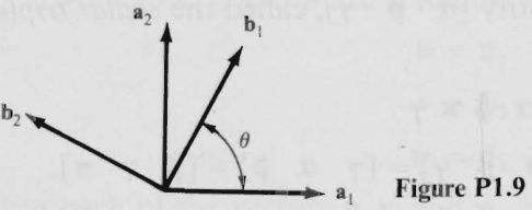
reference frame in which {\bf a}_{1} and {\bf a}_{2} are fixed, B a reference frame in which {\bf b}_{1} and {\bf b}_{2} are fixed, and \mathbf{v} a vector given by

\mathbf{v}=f\mathbf{a}_{1}+g\mathbf{a}_{2}

where f and g arefunctions of two scalar variables q_{1} and q_{2} ,showthat,if \theta is also afunctionof q_{1} and q_{2} ,then

\frac{{}^{A}\partial}{\partial q_{1}}\left(\frac{{}^{B}\partial{\bf v}}{\partial q_{2}}\right)-\frac{{}^{B}\partial}{\partial q_{2}}\left(\frac{{}^{A}\partial{\bf v}}{\partial q_{1}}\right)=\left(g{\bf a}_{1}\mathrm{~-~}f{\bf a}_{2}\right)\frac{\partial^{2}\theta}{\partial q_{1}\,\partial q_{2}}

1.10 A circular disk \textrm{C} of radius r can rotate about an axis X fixed in a laboratory L as shown in Fig.P1.10, and a rod R of length 3r is pinned to \textrm{C} ,the axis Y of the pin passing through the center \upsilon of {\cal C} Letting \mathbf{p} be the position vector from o to P ,the endpoint of R ,express the first time-derivative of \mathbf{p} in L in terms of q_{1},\,q_{2},\,\dot{q}_{1},\,\dot{q}_{2},\,{\bf c}_{1},\,{\bf c}_{2} , and \mathbf{c}_{3} ,where q_{1} and q_{2} are the radian measures of angles, as indicated in Fig. P1.9, \dot{q}_{1} and \dot{q}_{2} denote the time-derivatives of q_{1} and q_{2} , and \mathbf{c}_{1} ， \mathbf{c}_{2} ， \mathbf{c}_{3} are unit vectors fixed in C and directed as shown.

Suggestion:Firstverify that

\frac{{\bf\nabla}^{L}\hat{\sigma}{\bf c}_{2}}{\hat{\sigma}q_{1}}={\bf c}_{3}\qquad\frac{{\bf\nabla}^{L}\hat{\sigma}{\bf e}_{3}}{\hat{\sigma}q_{1}}={\bf\nabla}-{\bf c}_{2}

Result r[\dot{q}_{1}(\mathfrak{e}_{3}-3\,\sin q_{2}\mathfrak{e}_{2})+3\dot{q}_{2}(\cos q_{2}\mathfrak{e}_{3}+\sin q_{2}\mathfrak{e}_{1})]

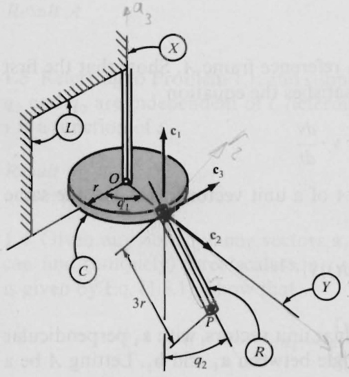
FigureP1.10

\mathbf{*1.11} A vector \mathbf{v} is a function of time t in a reference frame N in which mutually perpendicular unit vectors \mathbf{n}_{1},\mathbf{n}_{2},\mathbf{n}_{3} are fixed. At time t^{*}

\mathbf{v}=\mathbf{n}_{1}\qquad{\frac{N_{d}\mathbf{v}}{d t}}=\mathbf{n}_{2}\qquad{\frac{N_{d}^{2}\mathbf{v}}{d t^{2}}}=\mathbf{n}_{3}

Letting u be a unit vector that has the same direction as v at all times, determine themagnitude of ^N d^{2}\mathbf{u}/d t^{2} at time t^{*}

Result \sqrt{2}

PROBLEM SET 2

(Secs. 2.1-2.5)

2.1 When a point P moves on a space curve c fixed in a reference frame \pmb{A} a dextral set of orthogonal unit vectors \mathbf{b}_{1},\,\mathbf{b}_{2},\,\mathbf{b}_{3} can be generated by letting \pmb{\mathbb{p}} be the position vector from a point o fixed on c to the point P and defining \ensuremath{\mathbf{b}}_{1},\ensuremath{\mathbf{b}}_{2} , and {\bf b}_{3} as

\mathbf{b}_{1}\triangleq\mathbf{p}^{\prime}\qquad\mathbf{b}_{2}\triangleq\frac{\mathbf{p}^{\prime\prime}}{|\mathbf{p}^{\prime\prime}|}\qquad\mathbf{b}_{3}\triangleq\mathbf{b}_{1}\times\mathbf{b}_{2}

where primes denote differentiation in \pmb{A} with respect to the length s of the arc of c that connects o to P (see Fig. P2.1). The vector {\bf b}_{1} is called a vector tangent, {\bf b}_{2} the vector principal normal, and {\mathfrak{b}}_{3} a vector binormal of c at \pmb{P} , and the derivatives in \pmb{A} of \mathbf{b}_{1},\mathbf{b}_{2} , and {\bf b}_{3} with respect to \boldsymbol{s} are given by the Serret-Frenet formulas

\mathbf{b_{1}}^{\prime}={\frac{\mathbf{b_{2}}}{\rho}}\qquad\mathbf{b_{2}}^{\prime}=\,-\,{\frac{\mathbf{b_{1}}}{\rho}}+\lambda\mathbf{b_{3}}\qquad\mathbf{b_{3}}^{\prime}=\,-\,\lambda\mathbf{b_{2}}

where \rho and \lambda , defined as

\rho\triangleq{\frac{1}{|\mathbf{p}^{\prime\prime}|}}\qquad\lambda\triangleq\rho^{2}\mathbf{p}^{\prime}\cdot\mathbf{p}^{\prime\prime}\times\mathbf{p}^{\prime\prime\prime}

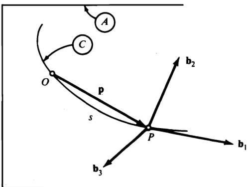
Figure P2.1

are called the principal radius of curvature of c at P and the torsion of c at \pmb{P} respectively.

Letting \pmb{B} be a rigid body in which \mathbf{b}_{1},\,\mathbf{b}_{2},\,\mathbf{b}_{3} are fixed, express the angular velocity of \pmb{B} in \pmb{A} in terms of \mathbf{b}_{1},\mathbf{b}_{2},\mathbf{b}_{3},\rho,\lambda, and \dot{s}, the time-derivative of \boldsymbol{s} , taking advantage of the fact that

\frac{{}^{A}d{\bf b}_{i}}{d t}={\bf b}_{i}{}^{\prime}\dot{s}\qquad(i=1,2,3)

Result (\lambda\mathbf{b}_{1}+\mathbf{b}_{3}/\rho)\dot{s}

2.2 Table P2.2 shows the relationship between two dextral sets of orthogonal unit vectors, {\bf a}_{1},{\bf a}_{2},{\bf a}_{3} and \ b_{1},\ b_{2},\ b_{3} , fixed in rigid bodies A and B_{\mathrm{i}} respectively. The symbols \mathbf{s}_{i} and \mathbf{c}_{i} in the table stand for sin q_{i} and cos q_{i} ,respectively,where q_{i}\,(i=1,2,3) are the radian measures of certain angles.

Table P2.2

<html>

	b1	b2	b3
a1	C2C3	SS2C3-S3C1	CS2C3+S3S1
a2	C2S3	SS2S3+C3C1	CS2S3-C3S1
a3	-S2	SC2	CC2

</html>

Determine {\mathfrak{x}}_{2} and \beta_{2} such that \mathbf{\delta}_{\mathbf{\theta}} , the angular velocity of \pmb{B} in \pmb{A} , is given by

\mathbf{\omega}\mathbf{\omega}=\alpha_{1}\mathbf{a}_{1}+\alpha_{2}\mathbf{a}_{2}+\alpha_{3}\mathbf{a}_{3}=\beta_{1}\mathbf{b}_{1}+\beta_{2}\mathbf{b}_{2}+\beta_{3}\mathbf{b}_{3}

Results \dot{q}_{1}\mathtt{c}_{2}\mathtt{s}_{3}+\dot{q}_{2}\mathtt{c}_{3}\qquad\dot{q}_{2}\mathtt{c}_{1}+\dot{q}_{3}\mathtt{s}_{1}\mathtt{c}_{2}

2.3 Referring to Problem 1.1, use the definition of angular velocity given in Sec. 2.1 to show that the angular velocity of \boldsymbol{B} in \boldsymbol{D} canbe expressed as

{\mathbf\Delta^{D}\!\mathbf{\dot{o}}^{B}}=\mathbf{\Phi}\!-\!(\dot{q}_{3}\sin q_{2}\,\mathbf{b}_{1}+\,\dot{q}_{2}\,\mathbf{b}_{2}+\,\dot{q}_{3}\cos q_{2}\,\mathbf{b}_{3})

Next, form \pmb{D_{\pmb{\upomega}}}\pmb{C_{\pmb{\upomega}}}\pmb{C_{\pmb{\upomega}}} and \pmb{c_{\pmb{\omega}}^{B}}_{\pmb{\omega}} , and then verify that ^D\!\mathbf{\omega}\!\!^{B}={^D\!\mathbf{\omega}\!\!\!^{C}}+{^c\!\mathbf{\omega}\!\!\!^{B}}, in agreement with the addition theorem for angular velocities. Finally, using the notations \mathbf{s}_{i}=\sin q_{i} ， \mathsf{c}_{i}=\mathsf{c o s}\,q_{i} (i=1,2,3) , determine \omega_{i} , defined as \omega_{i}\triangleq\omega^{D}\cdot\mathbf{d}_{i} (i=1,2,3)

\begin{array}{r}{\dot{q}_{1}\mathtt{c}_{2}\mathtt{c}_{3}+\dot{q}_{2}\,\mathtt{s}_{3}\qquad-\dot{q}_{1}\mathtt{c}_{2}\mathtt{s}_{3}+\dot{q}_{2}\mathtt{c}_{3}\qquad\dot{q}_{1}\mathtt{s}_{2}+\dot{q}_{3}}\end{array}

2.4 Letting w be the angular velocity of a rigid body B in a reference frame A, show that the angular velocity of A in B isequal to -\mathbf{\Gamma}\mathbf{\Gamma}\mathbf{\Gamma} and that

{\frac{{}^{A}d\mathbf{\omega}}{d t}}={\frac{{}^{B}d\mathbf{\omega}}{d t}}

*2.5 Letting β and β2 be nonparallel vectors fixed in a rigid body B, and using dots to denote differentiation with respect to time in a reference frame A, show that the angular velocity w of B in A can be expressed as

{\bf{\dot{o}}}=\frac{{\dot{\bf{\beta}}}_{1}\,{\bf\times}\,{\dot{\bf{\beta}}}_{2}}{{\dot{\bf{\beta}}}_{1}\cdot{\bf{\dot{{\beta}}}}_{2}}=\frac{1}{2}\left(\frac{{\dot{\bf{\beta}}}_{1}\,{\bf\times}\,{\dot{\bf{\beta}}}_{2}}{{\dot{\bf{\beta}}}_{1}\cdot{\bf{\beta}}_{2}}+\frac{{\dot{\bf{\beta}}}_{2}\,{\bf\times}\,{\dot{\bf{\beta}}}_{1}}{{\dot{\bf{\beta}}}_{2}\cdot{\bf{\beta}}_{1}}\right)

Suggestion: Make use of the fact that, for any vectors a, b, and c, a x (b x c) =a\cdot c b-a\cdot b c

2.6 Referring to Problem 2.1, suppose that q, the position vector from P to a point Q moving in A ,isgivenby

{\bf q}=q_{1}{\bf b}_{1}+q_{2}{\bf b}_{2}+q_{3}{\bf b}_{3}

where q_{1},\,q_{2},\,q_{3} are functions of time t_{\cdot} Determine the quantities v_{i}\;(i=1,2,3) such that the first time-derivative in A of the position vector r from O to Q is equal to v_{1}\mathbf{b}_{1}+v_{2}\mathbf{b}_{2}+v_{3}\mathbf{b}_{3}

Results \dot{q}_{1}+\dot{s}(1-q_{2}/\rho)\;\;\;\;\;\;\;\dot{q}_{2}+\dot{s}[(q_{1}/\rho)-\lambda q_{3}]\;\;\;\;\;\;\;\dot{q}_{3}+\dot{s}\lambda q_{2}

2.7 Figure P2.7 shows a circular disk C of radius R in contact with a horizontal plane H that is fixed in a reference frame A rigidly attached to the Earth. Mutually perpendicular unit vectors {\bf a}_{x},{\bf a}_{y} , and \mathbf{a}_{z}\triangleq\mathbf{a}_{x}\times\mathbf{a}_{y} are fixed in \pmb{A} , and \mathbf{b}_{1},\mathbf{b}_{2},\mathbf{b}_{3} form a dextral set of orthogonal unit vectors, with {\bf b}_{1} parallel to the tangent to the periphery of c at the point of contact between A and ^{c} {\bf b}_{2} parallel to the line connecting this contact point to C^{*} , the center of C_{v} and {\mathfrak{b}}_{3} normal to the plane of _{c}

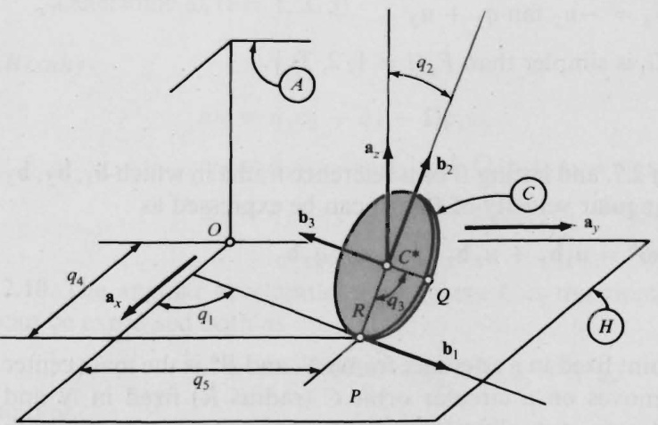
Figure P2.7

The orientation of c .n \pmb{A} can be described in terms of the three angles q_{1},q_{2},q_{3} indicated in Fig. P2.7, where Q is a point fixed on the periphery of c . The two quantities \mathbf{q_{4}} and q_{5} characterize the position in \pmb{A} of thepath point \pmb{P}

The angular velocity of C in \pmb{A} can be expressed both as

^{A}\!{\bf{\omega}}\!{\bf{\omega}}^{C}=u_{x}{\bf{a}}_{x}+u_{y}{\bf{a}}_{y}+u_{z}{\bf{a}}_{z}

and as

{\mathbf{\nabla}}^{A}\mathbf{\omega}^{C}=u_{1}\mathbf{b}_{1}+u_{2}\mathbf{b}_{2}+u_{3}\mathbf{b}_{3}

where u_{x},u_{y},u_{z} and u_{1},u_{2},u_{3} are functions of \pmb q_{i} and {\dot{q}}_{i} (i=1,2,3) .Concomitantly, {\dot{q}}_{i}\,(i=1,2,3) can be expressed as a function \boldsymbol{F}_{i} of q_{1},\,q_{2},\,q_{3},\,u_{x},\,u_{y},\,u_{z} or as a function G_{i}\,\mathrm{of}\,q_{1},q_{2},q_{3},u_{1},u_{2},u_{3}. Determine \boldsymbol{F}_{i} and G_{i} (i=1,2,3) ). [The equations {\dot{q}}_{i}=F_{i} and {\dot{q}}_{i}=G_{i} (i=1,2,3) are called kinematical differential equations. When u_{x},u_{y},u_{z} or u_{1},u_{2},u_{3} are known as functions of t_{\mathrm{:}} these equations can be solved for q_{1},q_{2},q_{3} to obtain a description of the orientation of c in A.]

Results

\begin{array}{r l}&{F_{1}=(-u_{x}s_{1}+u_{y}c_{1})\tan q}\\ &{F_{2}=-u_{x}c_{1}-u_{y}s_{1}}\\ &{F_{3}=(u_{x}s_{1}-u_{y}c_{1})\sec q_{2}}\\ &{G_{1}=u_{2}\sec q_{2}}\\ &{G_{2}=-u_{1}}\\ &{G_{3}=-u_{2}\tan q_{2}+u_{3}}\end{array}

[It is worth noting that G_{i} is simpler than F_{i}\,(i=1,2,3).]

2.8 Referring to Problem 2.7, and letting \pmb{B} be a reference frame in which \mathbf{b}_{1},\mathbf{b}_{2},\mathbf{b}_{3} are fixed, show that the angular velocity of \pmb{B} in \pmb{A} can be expressed as

^{A}\!{\mathfrak{w}}^{B}=u_{1}\mathbf{b}_{1}+u_{2}\,\mathbf{b}_{2}+u_{2}\tan q_{2}\,\mathbf{b}_{3}

2.9 In Fig. P2.9, o is a point fixed in a reference frame N , and B^{*} is the mass center of a rigid body \pmb{B} that moves on a circular orbit c (radius \pmb{R} ) fixed in N and centered at O.\;A_{1},\;A_{2},\;A_{3} are mutually perpendicular lines, A_{1} passing through o and B^{*} ， A_{2} tangent to c at B^{*} , and \boldsymbol{A}_{3} thus being normal to the plane of c

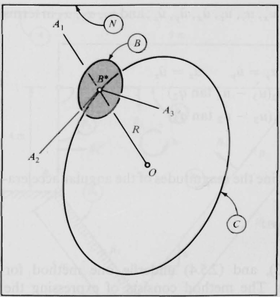
Figure P2.9

If {\bf b}_{1} {\bf b}_{2} {\bf b}_{3} form a dextral set of mutually perpendicular unit vectors fixed in B , the “attitude" of B in a reference frame A in which A_{1} A_{2} A_{3} are fixed can be specified in terms of q_{1},q_{2},q_{3} ,the radian measures of three angles generated as follows: Let {\bf a}_{1},\,{\bf a}_{2},\,{\bf a}_{3} be a dextral set of mutually perpendicular unit vectors fixed in A with \mathbf{a}_{i} parallel to A_{i}\,(i=1,2,3) , align \mathbf{b}_{i} with {\bf{a}}_{i} i=1 , 2, 3), and then subject B to successive right-handed rotations relative to A ,characterized by q_{1}\mathbf{b}_{1} \boldsymbol{q}_{2}\mathbf{b}_{2} ,and \boldsymbol{q}_{3}\mathbf{b}_{1} (note the last subscript). The quantities \omega_{i} (i=1,2,3 defined as

\omega_{i}\triangleq\mathbf{\omega}\cdot\mathbf{b}_{i}\qquad(i=1,2,3)

where \mathbf{\omega} is the angular velocity of B in N then can be expressed as functions of q_{i},\dot{q}_{i}\,(i=1,2,3) and \Omega if the angular velocity of A in N isgivenby \Omega\mathbf{a}_{3} Determine {\upsilon}_{i}\,(i=1,2,3)

Results

\begin{array}{r l}&{\omega_{1}=\dot{q}_{1}\mathtt{c}_{2}+\dot{q}_{3}-\Omega\mathtt{c}_{1}\mathtt{s}_{2}}\\ &{\omega_{2}=\dot{q}_{1}\mathtt{s}_{2}\mathtt{s}_{3}+\dot{q}_{2}\mathtt{c}_{3}+\Omega\left(\mathtt{c}_{1}\mathtt{c}_{2}\mathtt{s}_{3}+\mathtt{c}_{3}\mathtt{s}_{1}\right)}\\ &{\omega_{3}=\dot{q}_{1}\mathtt{s}_{2}\mathtt{c}_{3}-\dot{q}_{2}\mathtt{s}_{3}+\Omega(\mathtt{c}_{1}\mathtt{c}_{2}\mathtt{c}_{3}-\mathtt{s}_{3}\mathtt{s}_{1})}\end{array}

2.10 The angular acceleration \mathbf{\nabla}^{A}\mathbf{\alpha}^{C} where C is the circular disk in Problem 2.7, can be expressed both as

^{A}\pmb{\alpha}^{C}=\alpha_{x}\mathbf{a}_{x}+\alpha_{y}\mathbf{a}_{y}+\alpha_{z}\mathbf{a}_{z}

and as

{\mathbf{\nabla}}^{A}\pmb{\alpha}^{C}=\alpha_{1}\pmb{b}_{1}+\alpha_{2}\pmb{b}_{2}+\alpha_{3}\pmb{b}_{3}

Express \alpha_{x},\alpha_{y}, \mathfrak{X}_{z} in terms of q_{1},q_{2},q_{3},u_{x},u_{y},u_{z},\dot{u}_{x},\dot{u}_{y},\dot{u}_{z} ; and \pmb{\alpha}_{1},\,\pmb{\alpha}_{2}, {\mathfrak{a}}_{3} in terms of q_{i},\,u_{i},\,\dot{u}_{i}\,(i=1,2,3)

Results

\begin{array}{r l}&{\upalpha_{x}=\dot{u}_{x}\qquad\upalpha_{y}=\dot{u}_{y}\qquad\upalpha_{z}=\dot{u}_{z}}\\ &{\upalpha_{1}=\dot{u}_{1}+u_{2}(u_{3}-u_{2}\tan q_{2})}\\ &{\upalpha_{2}=\dot{u}_{2}-\dot{u}_{1}(u_{3}-u_{2}\tan q_{2})}\\ &{\upalpha_{3}=\dot{u}_{3}}\end{array}

2.11 Referring to Problem 1.10, determine the magnitudes of the angular acceleration of c in L,R in C , and \pmb R in L

Results |\ddot{q}_{1}|,|\ddot{q}_{2}|,[\ddot{q}_{1}^{2}+\ddot{q}_{2}^{2}+(\dot{q}_{1}\dot{q}_{2})^{2}]^{1/2} \bf{*2.12} Equations (2.1.2), (2.2.1), (2.5.3), and (2.5.4) underlie one method for analyzing motions of planar linkages. The method consists of expressing the position vector from a hinge point of the linkage to the same hinge point as the sum of position vectors from one hinge point to an adjacent one, setting this sum equal to zero, differentiating the resulting equation repeatedly with respect to.time t_{\mathrm{:}} , and making use of the relationships

A_{\pmb{\omega}^{B_{i}}}\quad=\quad\omega_{i}\mathbf{k}\qquad A_{\pmb{\alpha}^{B_{i}}}\quad=\quad\alpha_{i}\mathbf{k}

\begin{array}{c}{{\displaystyle\frac{{}^{A}\!\!\!-\!\!\!\!-\!\!\!}{d t}\!\!\!\!\!}}_{(2.1.2)}}\\ {{\displaystyle\frac{{}^{A}\!\!\!\!-\!\!\!\!}{d t}\!\!\!\!}}\\ {{\displaystyle\frac{d\!\!\!\!-\!\!\!\!-\!\!\!\!\!}{d t}\!\!\!\!\!}_{(2.1.2)}}\end{array}

and

\alpha_{i}\underset{(2.5.4)}{=}\frac{d\omega_{i}}{d t}

where \pmb{A} is a reference frame in which the plane of the linkage is fixed, B_{i} is a typical member of the linkage, \mathbf{k} is a unit vector normal to the plane of the linkage, \mathfrak{k}_{i} is a unit vector parallel to the line connecting the hinge points of B_{i},\mathfrak{b}_{i}^{\prime} is the unit vector {\textbf{k}}\times{\mathfrak{p}}_{i} , and \omega_{i} and \pmb{\alpha}_{i} are an angular speed of \pmb{B_{i}} (see Sec. 2.2) and a scalar angular acceleration of B_{i} (see Sec. 2.5), respectively.

Figure P2.12 shows the configuration at time t^{*} of a four-bar linkage, one bar of which, \pmb{{\cal B}_{4}} , is fixed in a reference frame \pmb{A} . At time t^{*} , the angular velocity of B_{3} in \pmb{A} and the angular acceleration of B_{1} in \pmb{A} are equal to -6\mathbf{k}\;\mathbf{rad/s} and \mathbf{5k} \mathbf{rad}/\mathbf{s}^{2} , respectively. Determine the angular velocities of B_{1} and B_{2} in \pmb{A} , and the angular accelerations of B_{2} and B_{3} in \pmb{A} , at time t^{*} , by making use of the equation

10\beta_{1}\,+\,9\beta_{2}\,+\,4\beta_{3}\,+\,5\beta_{4}=0

which is valid for all \boldsymbol{t}

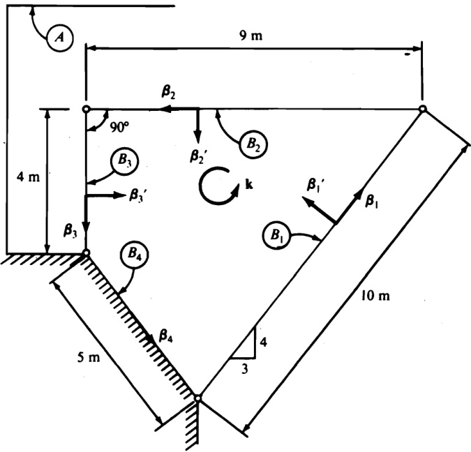
Figure P2.12

Results

\begin{array}{l l}{{{\cal A}_{\Theta}{}^{B_{1}}=\mathrm{-}\,{3}{\bf k}\ \mathrm{rad/s}\qquad\quad{}}}&{{{\cal A}_{\Theta}{}^{B_{2}}=\mathrm{-}\,{2}{\bf k}\ \mathrm{rad/s}\ }}\\ {{{\cal A}_{\alpha}{}^{B_{2}}=(34/3){\bf k}\ \mathrm{rad/s}{}^{2}\qquad{\cal A}_{\alpha}{}^{B_{3}}=(29/2){\bf k}\ \mathrm{rad/s}{}^{2}}}\end{array}

PROBLEM SET 3

(Secs. 2.6-2.8)

3.1 Apply the definitions given in Eqs. (2.6.1) and (2.6.2) to formulate expressions for the velocity and the acceleration of the endpoint \pmb{P} of the rod \pmb R of Problem 1.10 in (a) reference frame \pmb{L} and (b) the circular disk c

Results

\begin{array}{r l}&{^{L}\mathbf{v}^{P}=r[3\sin q_{2}(\dot{q}_{2}\mathbf{c}_{1}-\dot{q}_{1}\mathbf{c}_{2})+(\dot{q}_{1}+3\dot{q}_{2}\cos q_{2})\mathbf{c}_{3}]}\\ &{^{L}\mathbf{a}^{P}=r\{3(\ddot{q}_{2}\sin q_{2}+\dot{q}_{2}{}^{2}\cos q_{2})\mathbf{c}_{1}}\\ &{\phantom{^L}\;\;\;\;\;\;\;-{\left(3\ddot{q}_{1}\sin q_{2}+6\dot{q}_{1}\dot{q}_{2}\cos q_{2}+\dot{q}_{1}{}^{2}\right)}\mathbf{c}_{2}}\\ &{\phantom{^L}\;\;\;\;\;\;\;+{\left[\ddot{q}_{1}+3\ddot{q}_{2}\cos q_{2}-3(\dot{q}_{1}{}^{2}+\dot{q}_{2}{}^{2})\sin q_{2}\right]}\mathbf{c}_{3}\}}\\ &{^{c}\mathbf{v}^{P}=3r\dot{q}_{2}(\sin q_{2}\mathbf{c}_{1}+\cos q_{2}\mathbf{c}_{3})}\\ &{^C\mathbf{a}^{P}=3r[(\ddot{q}_{2}\sin q_{2}+\dot{q}_{2}{}^{2}\cos q_{2})\mathbf{c}_{1}+(\ddot{q}_{2}\cos q_{2}-\dot{q}_{2}{}^{2}\sin q_{2})\mathbf{c}_{3}]}\end{array}

3.2 A point \pmb{P} moves on a space curve c fixed in a reference frame A. Show that \mathbf{v}. the velocity of \pmb{P} in \pmb{A} , can be expressed as

where {\bf b}_{1} is a vector tangent of C at P (see Problem 2.1), and verify that a, the acceleration of P in A , is given by

{\bf a}=\dot{v}{\bf b}_{1}+{\frac{v^{2}}{\rho}}\,{\bf b}_{2}

where {\bf b}_{2} and \rho are, respectively, the vector principal normal and the principal radius of curvature of C at P

3.3 Letting u_{4}\triangleq\dot{q}_{4} and u_{5}\triangleq\dot{q}_{5} ,with \mathbf{q_{4}} and \pmb q_{5} defined as in Problem 2.7, determine v_{i}\,(i=1,2,3) such that the velocity of C^{*} in \pmb{A} is given by

^{A}\mathbf{v}^{C^{*}}=v_{1}\mathbf{b}_{1}+v_{2}\mathbf{b}_{2}+v_{3}\mathbf{b}_{3}

Express v_{i}\,(i=1,2,3) as functions of \pmb q_{j} and u_{j}\,(j=1,\ldots,5)

Results

\begin{array}{r l}&{v_{1}=\,-R u_{2}\,\tan\,q_{2}\,+\,u_{4}c_{1}\,+\,u_{5}s_{1}}\\ &{v_{2}=(-u_{4}s_{1}\,+\,u_{5}c_{1})s_{2}}\\ &{v_{3}=R u_{1}\,+\,(u_{4}s_{1}\,-\,u_{5}c_{1})c_{2}}\end{array}

3.4 If a_{i} is defined as a_{i}\triangleq\mathbf{\mathcal{A}}_{\mathbf{a}}c^{\ast}\cdot\mathbf{b}_{i} (i=1,2,3) ,where A and C^{*} have the same meaning as in Problem 2.7 and \mathbf{\Psi_{a}}\mathbf{c}^{\bullet} denotes the acceleration of C^{\ast} in \pmb{A} , then a_{1},a_{2},a_{3} can be expressed as functions of \boldsymbol{q}_{j},\,\boldsymbol{u}_{j} and \dot{u}_{j}\,(j=1,\dotsc,5) , with \pmb{u_{4}} and \pmb{u}_{5} defined as in Problem 3.3. Determine these functions.

Results

\begin{array}{r l}&{a_{1}=-\dot{u}_{2}R\operatorname{tan}{q_{2}}+\dot{u}_{4}\mathtt{c}_{1}+\dot{u}_{5}\mathtt{s}_{1}+u_{1}u_{2}R(1+\mathtt{s e c}_{1})}\\ &{a_{2}=(-\dot{u}_{4}\mathtt{s}_{1}+\dot{u}_{5}\mathtt{c}_{1})\mathtt{s}_{2}-R{u_{1}}^{2}-R{u_{2}}^{2}\tan^{2}{q_{2}}}\\ &{a_{3}=\dot{u}_{1}R+(\dot{u}_{4}\mathtt{s}_{1}-\dot{u}_{5}\mathtt{c}_{1})\mathtt{c}_{2}+{u_{2}}^{2}R\operatorname{tan}{q_{2}}}\end{array}

\bf{*}_{3.5} Determine the velocity \mathbf{v} and the acceleration a of the midpoint of bar B_{2} of the linkage described in Problem 2.12 for time t^{*}

\mathbf{v}=\,-\,24\mathsf{\pmb{\beta}}_{2}\,+\,9\mathsf{\pmb{\beta}}_{3}\,\mathbf{m}/\mathsf{s}\qquad\mathbf{a}\,=\,76\mathsf{\pmb{\beta}}_{2}\,+\,93\mathsf{\pmb{\beta}}_{3}\,\mathbf{m}/\mathsf{s}^{2}

3.6 At time t , there exists precisely one point of the disk c of Problem 2.7 (see also Problems 2.8, 2.10, 3.3, and 3.4) that is in contact with the plane \pmb{H} . Calling this point {\hat{C}}_{:} one can express the velocity and the acceleration of \hat{c} in \pmb{A} at time t as

^{A}\mathbf{v}^{\hat{c}}=\hat{v}_{x}\mathbf{a}_{x}+\hat{v}_{y}\mathbf{a}_{y}

and

{\mathbf{\nabla}}^{A}\mathbf{a}^{\hat{C}}=\hat{a}_{1}\mathbf{b}_{1}+\hat{a}_{2}\mathbf{b}_{2}+\hat{a}_{3}\mathbf{b}_{3}

respectively, where \hat{v}_{x} and \hat{v}_{y} are functions of \pmb q_{j} and u_{j}\ (j=1,\ldots,5) , and \hat{\pmb{a}}_{i} (i=1,2,3) are functions of \boldsymbol{q}_{j},\,\boldsymbol{u}_{j} and \dot{u}_{j}\,(j=1,\dotsc,5) Determine \hat{v}_{x},\,\hat{v}_{y} , and \hat{a}_{i}\,(i=1,2,3)

Suggestion: Use Eqs. (2.7.1) and (2.7.2), replacing the symbols P,Q_{\mathrm{i}} and \textbf{\emph{B}} with \hat{C},C^{\ast} and c respectively.

Results

\begin{array}{r l}&{\hat{v}_{x}=(-u_{2}\tan q_{2}+u_{3})R c_{1}+u_{4}}\\ &{\hat{v}_{y}=(-u_{2}\tan q_{2}+u_{3})R s_{1}+u_{5}}\\ &{\hat{a}_{1}=-\dot{u}_{2}R\tan q_{2}+\dot{u}_{3}R+\dot{u}_{4}c_{1}+\dot{u}_{5}s_{1}+u_{1}u_{2}R\sec^{2}q_{2}}\\ &{\hat{a}_{2}=(-\dot{u}_{4}s_{1}+\dot{u}_{5}c_{1})s_{2}+R({u_{3}}^{2}-u_{2}^{2}\tan^{2}q_{2})}\\ &{\hat{a}_{3}=(\dot{u}_{4}s_{1}-\dot{u}_{5}c_{1})c_{2}+2R u_{2}(u_{2}\tan q_{2}-u_{3})}\end{array}

3.7 Suppose that the quantities \hat{v}_{x} and \hat{v}_{y} of Problem 3.6 are differentiated with respectto t_{\mathrm{{}}} , the results are used to form a vector a defined as

\mathbf{a}\triangleq\frac{d\hat{v}_{x}}{d t}\,\mathbf{a}_{x}+\frac{d\hat{v}_{y}}{d t}\,\mathbf{a}_{y}

and quantities \overline{{{a}}}_{i}\left(i=1,2,3\right) then are formed as

\bar{a}_{i}\triangleq\mathbf{a}\cdot\mathbf{b}_{i}\qquad(i=1,2,3)

Do you expect \overline{{\pmb{a}}}_{i} to be equal to the quantity \pmb{\hat{a}}_{i} of Problem 3.6? First explain your answer, then establish its validity by determining \overline{{a}}_{i}\,(i=1,2,3)

3.8 If \pmb{\hat{A}} is a point of a rigid body A,\hat{B} a point of a rigid body B, \pmb{\hat{A}} and \pmb{\hat{B}} are in contact with each other at time \pmb{t}_{:} . and the velocities of \pmb{\hat{A}} and \pmb{\hat{B}} in any reference frame are equal to each other at time \pmb{t}, then \pmb{A} and \pmb{B} are said to be rolling on each other at time t. Alternatively, one can say that no slipping is taking place at the contact between \pmb{A} and \pmb{B} at time t. (If \pmb{A} and \pmb{B} are in contact with each other at more than one point, these contacts must be considered separately. The bodies \pmb{A} and \pmb{B} can be rolling on each other at some points while slipping is taking place at other points.)

When the circular disk ^{c} of Problem 2.7 rolls on plane \pmb{H} the quantities \pmb{u_{4}} and \pmb{u_{5}} of Problem 3.3 can be expressed as functions of {q_{j}}\;(j=1,\ldots,5) and u_{k}\,(k=1,2,3) . Determine these functions.

u_{4}=(u_{2}\ {\tan\,q_{2}-u_{3}})R\mathbf{c}_{1}\qquad u_{5}=(u_{2}\ {\tan\,q_{2}-u_{3}})R\mathbf{s}_{1}

3.9 When the circular disk C of Problem 2.7 rolls on plane H ,there exists at each instant one point \hat{C} of C that is in contact with H_{\mathrm{~\,~}} The acceleration of \hat{C} in A is not, in general, equal to zero. Express the magnitude of this acceleration in terms of R u_{2},u_{3} , and \dot{q}_{3}

Result R\,|\dot{q}_{3}|(u_{2}{}^{2}+u_{3}{}^{2})^{1/2}

3.10 When two rigid bodies A and B are rolling on each other (see Problem 3.8), the angular velocity \mathbf{\omega}^{A}\mathbf{\omega_{GD}}^{B} of B in A generally is not parallel to the plane P that is tangent to the surfaces of A and B at their points of contact with each other. When A_{\mathbf{Q}\mathbf{)}^{B}} is parallel to P , one speaks of pure rolling of A and B on each other.

FigureP3.10 shows a shaft terminating in a truncated cone C of semivertex angle \theta \mathrm{~0~}<\theta<\pi/4 rad),this shaft being supported by a thrust bearing consisting of a fixed race R and four identical spheres s of radius r When the shaftrotates, rolling takesplace atthe two contactsbetween R and S,as well as at the contact between s and C Moreover, s and C perform a pure rolling motion on each other (which is desirable because it minimizes wear) if the dimension ^b is a suitable function of r and \theta. Find thisfunction.

Result r(1+\sin\theta)/(\cos\theta-\sin\theta)

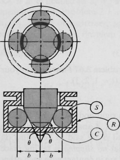
Figure P3.10

3.11 The concept of rolling (see Problem 3.8) comes into play in connection with gearing, where it can be invoked in conjunction with Eqs. (2.7.1) and (2.4.1) to discover relationships between angular speeds (see Sec. 2.2) of gears.

Figure P3.11 shows schematically how the drive shaft D of an automobile can be connected to the two halves, A and A^{\prime} of an axle in such a way as to permit wheels attached rigidly to _A and A^{\prime} to rotate at different rates relative to the frame F that supports D,\,A ,and A^{\prime} .This is accomplished as follows: Bevel gears B

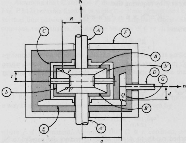
Figure P3.11

and B^{\prime} keyed to A and A^{\prime} ,respectively, engage bevel gears b and b^{\prime} , respectively; b and b^{\prime} are free to rotate on pins fixed in a casing C that can rotate about the (common) axis of A and A^{\prime} and a bevel gear E ,fastenedrigidlyto \textrm{\textbf{C}} ,is driven by a bevel gear G thatiskeyedto D

Letting P,\,P^{\prime} ,and Q be points selected arbitrarily on the lines of contact between B and b B^{\prime} and b and G and E respectively, and assuming that rolling is taking place at these points, one can discover the relationship between angular speeds F_{\omega}^{\quad A\quad F}\omega^{A^{\prime}} ,and {}^{F}\!_{C\!\!\!\!/\!\!\!/\!\!\!\!/}{D} defined as

{}^{F}\!\omega^{A}\:\triangle\ {}^{F}\!{\bf0}\!\cdot\!{\bf N}\qquad{}^{F}\!\omega^{A^{\prime}}\:\triangle\ {}^{F}\!{\bf0}\!\cdot\!{\bf N}\qquad{}^{F}\!_{G}\!\!)^{D}\:\triangle\ {}^{F}\!{\bf0}\!\cdot\!{\bf n}

where \mathbf{N} and \mathbf{n} are unit vectors directed as shown in Fig. P3.11, by reasoning as follows.

B and b have simple angular velocities in C and,after expressing these as

^{C}{\bf{\omega}}{^{B}}=^{C}\!\omega^{B}{\bf{N}}\quad\quad{^{C}}{\bf{\omega}}{^{b}}={^{C}}\!\omega^{b}{\bf{n}}

onecanlet \hat{B} and \hat{b} be the points of B and b respectively, that come into contact at P ;introduce distances R and r as shown in Fig.P3.11;write for the velocities of \hat{B} and \hat{b} in C

\begin{array}{c c c}{{c_{\mathbf{v}}\hat{\pmb{\theta}}}}&{{=}}&{{c_{\mathbf{0}}\pmb{\theta}^{B}\,\times\,(-\,R\,\mathbf{n})=\,-\,R^{C}\omega^{B}\mathbf{N}\,\times\,\mathbf{n}}}\end{array}

and

\begin{array}{r l r}{c_{\pmb{\Psi}}^{~\hat{b}}}&{{}=}&{c_{\pmb{\omega}}^{~c}\pmb{\omega}^{b}\,\times\,(r\mathbf{N})=r^{C}\omega^{b}\pmb{\mathfrak{n}}\,\times\,\mathbf{N}}\end{array}

and then ensure rolling at P by requiring that

-R^{c}\omega^{B}\mathbf{N}\times\mathbf{n}=r^{c}\omega^{b}\mathbf{n}\times\mathbf{N}

which is guaranteed when

R^{\mathrm{{c}}}\omega^{B}=r^{\mathrm{{c}}}\omega^{b}

Similarly, by taking rolling at P^{\prime} and at Q into account, one arrives at relationships between c_{\omega^{B^{\prime}}} , and c_{\omega^{b}} , in one case, and {}^{F}{}_{O^{j}}{}^{E} and F_{\omega}\omega ,in the other case, where c_{\omega^{B^{\prime}}} \hat{\boldsymbol{r}}_{O^{2}}\hat{\boldsymbol{\varepsilon}} , and F_{(\!\!\cdot\!\!\!)}\mathrm{c} are angular speeds defined in terms of associated angular velocitiesas

{{{c}_{{\cal O}}}{{}^{B^{\prime}}}}\,\triangleq\,{{{c}_{{\bf0}}}{{}^{B^{\prime}}}}\cdot{{\bf N}}\qquad{{{}^{F}}{_{{\cal O}}}{{}^{E}}}\,\triangleq\,{{{}^{F}}{_{{\bf0}}}{{}^{E}}}\cdot{{\bf N}}\qquad{{}^{F}}{_{{\cal O}}}{{}^{G}}\,\triangleq\,{{{}^{F}}{_{{\bf0}}}{{}^{G}}}\cdot{{\bf n}}

Next, one has

{}^{F}\mathbf{\omega}_{\mathbf{0}}^{B}~~~=~~{}^{F}\mathbf{\omega}_{\mathbf{0}}^{C}+{}^{c}\mathbf{\omega}^{B}

which, since B is attached rigidly to A , and all three vectors are parallel to \mathbf{N} implies that

{}^{F}\!\omega^{A}={}^{F}\!\omega^{C}+{}^{c}\omega^{B}

where \begin{array}{r}{{\cal F}_{\omega}c\triangleq{\cal F}_{\omega}c\cdot{\bf N}.}\end{array} Using Eq. (2.4.1) once more, this time in connection with B^{\prime},\ C and F , then brings one into position to find the relationship between Fo4, Fo4', and FoD by purely algebraic means.

Show that

{}^{F}\omega^{D}=\frac{a}{2d}\,({}^{F}\omega^{A}\,+\,{}^{F}\omega^{A^{\prime}})

3.12 Figure P3.12 shows a right-circular, uniform, solid cone C in contact with ahorizontalplane P thatis fixed in areference frame A The base of C hasa radius R and C has a height 4h

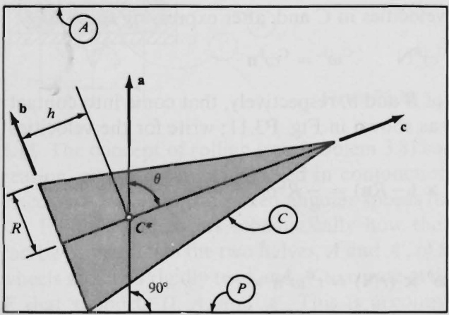
Figure P3.12

Assuming that c rolls on \pmb{P} in such a way that the mass center c^{*} of c (see Fig. P3.12) remains fixed in \pmb{A} while the plane determined by the axis of c and a vertical line passing through C^{*} has an angular velocity \pmb{\Omega} in \pmb{A} ,where \pmb{\Omega} is a constant, verify that \pmb{\omega} , the angular velocity of ^{c} in \pmb{A} ,is given by

\mathbf{0}=\Omega s\theta\biggl(\mathbf{b}+\frac{h}{R}\,\mathbf{c}\biggr)

where \theta is the inclination angle of the axis of c while a, \begin{array}{r}{\mathbf{b},}\end{array} . and c are unit vectors directed as shown in Fig. P3.12.

3.13 Referring to Problem 2.9, let \pmb{P} be a particle that moves on body \pmb{B} in such a way that the position vector r from B^{*} to \pmb{P} is given by

\mathbf{r}=c(\Omega^{2}t^{2}-1)\mathbf{b}_{3}

where ^c is a constant. Assuming that \pmb{\Omega} is a constant, and letting q_{1}=q_{2}= q_{3}=\pi/2 rad at time t=1/\Omega determine the acceleration of \pmb{P} in N for this instant.

Result 4c\Omega\dot{q}_{1}\mathbf{b}_{1}-\Omega(R\Omega+4c\dot{q}_{3})\mathbf{b}_{2}+2c\Omega^{2}\mathbf{b}_{3}

3.14 The path point \pmb{P} mentioned in Problem 2.7 has a velocity both in \pmb{A} and in c , and these velocities can be expressed as

^A\mathbf{v}^{P}=\tilde{v}_{x}\mathbf{a}_{x}+\tilde{v}_{y}\mathbf{a}_{y}+\tilde{v}_{z}\mathbf{a}_{z}

and

c_{\mathbf{v}}P=\tilde{v}_{1}\mathbf{b}_{1}+\tilde{v}_{2}\mathbf{b}_{2}+\tilde{v}_{3}\mathbf{b}_{3}

respectively, where \tilde{v}_{x},~\tilde{v}_{y},~\tilde{v}_{z} , and \tilde{v}_{i} (i=1,2,3) are functions of \pmb q_{j} and \pmb{u}_{j} (j=1,\ldots,5) ,with \pmb{u_{4}} and \pmb{u_{5}} defined as in Problem 3.3. Determine \tilde{v}_{x},\,\tilde{v}_{y},\,\tilde{v}_{z},\,\tilde{v}_{i}, and \tilde{a}_{i}\,(i=1,2,3) , with \tilde{\pmb{a}}_{i} defined as

\tilde{a}_{i}\triangleq c_{\mathbf{a}}\boldsymbol{r}\cdot\mathbf{b}_{i}\qquad(i=1,2,3)

where c_{\mathbf{a}^{P}} is the acceleration of \pmb{P} in c

Suggestion: To find c_{\mathbf{v}^{P}} and c_{\mathbf{a}^{P}} , use Eqs. (2.8.1) and (2.8.2), replacing \pmb{B} with C_{v} and \bar{\pmb{B}} with \hat{c} as defined in Problem 3.6.

Results

\begin{array}{l}{{\tilde{v}_{x}=u_{4}\qquad\tilde{v}_{y}=u_{5}\qquad\tilde{v}_{z}=0}}\\ {{\tilde{v}_{1}=R(u_{2}\,\tan q_{2}-u_{3})\qquad\tilde{v}_{2}=\tilde{v}_{3}=0}}\\ {{\tilde{a}_{1}=R(\dot{u}_{2}\,\tan q_{2}-\dot{u}_{3}-u_{1}u_{2}\,\sec^{2}q_{2})}}\\ {{\tilde{a}_{2}=R(u_{2}\,\tan q_{2}-u_{3})^{2}}}\\ {{\tilde{a}_{3}=0}}\end{array}

^{*}3.15 Figure P3.15 is a schematic representation of a robot arm consisting of three elements A B ,and \textit{C} ,the last of which holds a rigid body D rigidly. One end of A is ahub that is made torotate about avertical axisfixed in theEarth E At a point P,B is connected to A by means of a motor (all parts of which are rigidly attachedeitherto A orto B )thatcauses B torotaterelativeto A aboutahorizontal axis fixed in A ,passing through P ,and perpendicular to the axisof A .Finally, \textrm{C} is connected to B bymeans of arack-and-pinion drive thatcanmake \textrm{C} slide relative to B

Letting L_{A} ， L_{B} , and L_{P} denote distances as indicated in Fig. P3.15, where
A^{*},B^{*} ,and C^{*} are points fixed on A,B ,and \mathbb{C} , respectively, introduce unit vectors
\mathbf{a}_{i} and \mathbf{\bar{D}}_{i} (i = 1, 2, 3) as shown in Fig. P3.15, let p_{i}\triangleq\mathbf{p}^{C^{*}D^{*}}\cdot\mathbf{b}_{i} ,where \mathfrak{p}^{\mathbb{C}^{*\!p*}} is the
position vector from C^{*} to D^{*} ,the mass center of D ,and define ， ， as \boldsymbol{u}_{1} u_{2} u_{3}

u_{1}\triangleq^{E}\!\mathbf{0}^{A}\cdot\mathbf{a}_{1}\qquad u_{2}\triangleq^{A}\!\mathbf{0}^{B}\cdot\mathbf{b}_{2}\qquad u_{3}\triangleq^{B}\!\mathbf{v}^{C^{\ast}}\!\cdot\mathbf{b}_{3}

where \varepsilon_{\mathbf{G}^{A}} is the angular velocity of A in E \mathbf{\Pi}^{A}\mathbf{\Pi}_{[0)}\mathbf{\tilde{\mathbf{\Pi}}}^{B} is the angular velocity of B in A and {\boldsymbol{s}}_{\boldsymbol{\mathbf{\check{v}}}}{\boldsymbol{c}}^{*} is the velocity of C^{*} in B . Denoting the radian measure of the angle between the axes of A and B by q_{1} ,letting \mathrm{s}_{1}\triangleq sin q_{1} \mathtt{c}_{1}\triangleq cOS q_{1} and designating as q_{2} the distance from B^{*} to C^{*} , determine \varepsilon_{\mathbf{60}^{A}} \boldsymbol{E}_{\mathbf{0}\mathbf{0}}B \varepsilon_{\mathbf{o}}c and \varepsilon_{\mathbf{\omega}}\mathbf{\rho}_{\mathbf{G}}p_{\mathbf{\rho}} , the angular velocities of A B \textrm{C} ,and \boldsymbol{D} in E;{}^{E}{\pmb{\alpha}}^{A} \varepsilon_{\pmb{\alpha}^{B}} \varepsilon_{\pmb{\alpha}^{C}} and \boldsymbol{\varepsilon}_{\pmb{\alpha}^{D}} the angular accelerations of A B C ,and D in E;\,{}^{t}\mathbf{v}^{A^{*}} {\boldsymbol{\varepsilon}}_{\mathbf{V}}{\boldsymbol{B}}^{*} {\mathbf{\mathit{\varepsilon}}}_{{\mathbf{\mathit{\varepsilon}}}{\mathbf{\mathit{\varepsilon}}}}^{\varepsilon} ,and {\boldsymbol{E}}_{\mathbf{V}}{\boldsymbol{D}}^{*} the velocities of A^{*},B^{*},C^{*}, and D^{*} in E ; and ^{E}\mathbf{a}^{A^{*}},^{E}\mathbf{a}^{B^{*}},^{E}\mathbf{a}^{C^{*}} and \mathbf{\boldsymbol{\varepsilon}}_{\mathbf{a}}\mathbf{\boldsymbol{\nu}}^{*} the accelerations of A^{*} B^{*} C^{*} and D^{*} E (Note that \dot{q}_{1}=u_{2} and \dot{q}_{2}=u_{3}

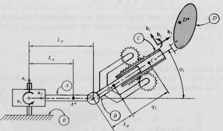
Figure P3.15

Suggestion: To facilitate the writing of results, introduce Z_{1},...,Z_{34} as

\begin{array}{r l}&{Z_{1}\triangleq u_{1}c_{1},\quad Z_{2}\triangleq u_{1}s_{1},\quad Z_{3}\triangleq-Z_{2}u_{2},\quad Z_{4}\triangleq Z_{1}u_{2},\quad Z_{5}\triangleq-L_{4},}\\ &{Z_{6}\triangleq-(L_{+}+L_{\delta^{\star}\times1})\quad Z_{7}\triangleq u_{2}L_{\delta},\quad Z_{8}\triangleq\pm Z_{6}u_{1},\quad Z_{9}\triangleq L_{8}+q_{2},}\\ &{Z_{10}\triangleq Z_{6}-q_{2}c_{1},\quad Z_{11}\triangleq u_{2}Z_{9},\quad Z_{12}\triangleq Z_{10}u_{1},\quad Z_{13}\triangleq-s_{1}p_{2}}\\ &{Z_{14}\triangleq Z_{9}+p_{3},\quad Z_{15}\triangleq Z_{10}+s_{1}p_{1}-\varsigma_{19},\quad Z_{16}\triangleq c_{1}p_{2}}\\ &{Z_{17}\triangleq Z_{18}u_{1}+Z_{14}u_{2},\quad Z_{18}\triangleq\pm Z_{19}u_{1}\quad Z_{19}\triangleq Z_{16}u_{1}-u_{2}P_{1}+u_{3}}\\ &{Z_{20}\triangleq u_{1}Z_{5},\quad Z_{21}\triangleq L_{8}s_{10},\quad Z_{22}\triangleq-Z_{2}z_{8}\quad Z_{23}\triangleq Z_{21}u_{1}+Z_{2}z_{1}}\\ &{Z_{24}\triangleq Z_{15}-u_{2}Z_{7},\quad Z_{25}\triangleq Z_{21}-u_{3}c_{1}+q_{2}s_{12}}\\ &{Z_{26}\triangleq2u_{2}u_{3}-Z_{2}z_{12},\quad Z_{27}\triangleq Z_{25}u_{1}+Z_{2}z_{11}-Z_{14}u_{3}}\\ &{Z_{28}\triangleq Z_{1}Z_{12}-u_{2}Z_{11},\quad Z_{29}\triangleq-Z_{16}u_{2}\quad Z_{30}\triangleq Z_{25}+u_{2}(c_{1}P_{1}+s_{1})}\\ &{Z_{31}\triangleq Z_{13}u_{2},\quad Z_{32}\triangleq Z_{29}

Results

\begin{array}{r l}&{\mathrm{~\partial_{t}\phi^\nu=}u_{11}}\\ &{\mathrm{~\partial_{t}\phi^\nu=}\;\delta_{0}^{\phantom{\nu}}=\mathrm{\partial_{\theta}}v=u_{1}\mathrm{\partial_{t}\phi_{1}}+u_{2}\mathrm{\partial_{\phi}}+u_{1}\mathrm{\partial_{b}}\mathrm{\partial_{x}}=Z_{1}\mathrm{b_{1}}+u_{2}\mathrm{\partial_{\phi}}+Z_{2}\mathrm{b_{2}}}\\ &{\mathrm{~\partial_{t}\phi^\nu=}\;\delta_{1,1}^{\phantom{\nu}}\;\;\;\;\varepsilon_{\alpha}^{\alpha}=\mathrm{\partial_{\theta}}v=(u_{1}\mathrm{\partial_{c}1}+Z_{2})\mathrm{b_{1}}+\mathrm{\partial_{z}\phi_{2}}+(u_{1}\mathrm{\partial_{x}}+Z_{2})\mathrm{\partial_{z}\phi_{1}}}\\ &{\mathrm{~\partial_{t}\phi^\nu=}\;-L_{\mathrm{a}}u_{1,2}\mathrm{\partial_{z}}=Z_{3,2}\mathrm{\partial_{t}\phi_{1}^{\nu}}-u_{2,L_{\mathrm{a}}\mathrm{\partial_{b}}}\mathrm{\partial_{z}}+Z_{6,u_{1}\mathrm{\partial_{z}}}=Z_{\mathrm{b_{1}}}+Z_{8}\mathrm{\partial_{z}}}\\ &{\mathrm{~\partial_{t}\phi^{\nu}=}\;u_{2}\mathrm{\partial_{b}1}+Z_{1,0}u_{1}\mathrm{\partial_{z}}+u_{3}\mathrm{\partial_{b}3}=Z_{1,1}\mathrm{\partial_{t}\phi_{1}}+Z_{1,0}\mathrm{\partial_{z}}+u_{3}\mathrm{\partial_{b}}}\\ &{\mathrm{~\partial_{t}\phi^\nu=}\;(\mathrm{\partial_{z1}u_{1}}+Z_{1,1}u_{2}\mathrm{\partial_{b}1}+Z_{1,1}u_{1}\mathrm{\partial_{z}}+(Z_{1}u_{1}-u_{2}\mathrm{\partial_{P}1}+u_{3})\mathrm{\partial_{b}},}\\ &{\mathrm{~\partial_{t}\phi_{1}^{\nu}=}\;{Z_{1,0}b_{1}+Z_{1,1}b_{2}+Z_{1,9}b_{3}} 

Note that two expressions are given for the angular velocities of B,\,C. , and \pmb{D} in {\pmb E}_{\mathrm{~\,~}} , as well as for the velocities of A^{*},\,B^{*},\,C^{*} , and D^{*} in {\pmb E} . In each case, the quantities u_{1},\,u_{2},\,u_{3} appear explicitly in the first expression but are absent from the second, except in the case of \pmb{\varepsilon_{v}}\pmb{c_{\nu}^{\star}} , where no simplification would result from replacing \pmb{u}_{3} with another symbol. There are two reasons for writing each angular velocity and each velocity in these two ways. The first will become apparent in connection with Problem 4.17; the second is that both versions come into play when one seeks to write expressions for angular accelerations of rigid bodies and accelerations of mass centers in such a way that \dot{\pmb u}_{1},\dot{\pmb u}_{2} , and \dot{u}_{3} appear explicitly.

PROBLEM SET 4

(Secs. 2.9-2.15)

4.1 Mutually perpendicular unit vectors {\bf a}_{1},{\bf a}_{2} , and \mathbf{a}_{3}\triangleq\mathbf{a}_{1}\times\mathbf{a}_{2} are fixed in a reference frame \pmb{A} , and a unit vector b is fixed in a rigid body \boldsymbol{B} , one of whose points, o , is fixed in A,B is brought into a general orientation in \pmb{A} , after \mathbf{b} has been aligned with {\bf a}_{1} , by being subjected to successive rotations characterized by the vectors \theta_{1}\mathbf{a}_{1},\,\theta_{2}\mathbf{a}_{2} , and \theta_{3}\mathbf{a}_{3} , where \theta_{1},\,\theta_{2} , and \theta_{3} are the radian measures of angles. A particle P is free to move on a line L that is fixed in \pmb{B} passes through o and is parallel to b.

Letting \pmb{\mathbb{p}} be the position vector from o to P , and defining x_{i} as

x_{i}\triangleq\mathbf{p}\cdot\mathbf{a}_{i}\qquad(i=1,2,3)

show that \pmb{P} is guaranteed to remain on L when x_{1},x_{2} , and x_{3} satisfy the holonomic constraint equations

x_{1}s_{3}-x_{2}\mathbf{c}_{3}=0\qquad x_{3}\mathbf{c}_{2}\mathbf{c}_{3}+x_{1}\mathbf{s}_{2}=0

where \mathbf{s}_{i}\triangleq sin \theta_{i} \mathsf{c}_{i}\triangleq cOS \theta_{i}\,(i=2,3)

Letting \pmb q be an arbitrary quantity, verify that the constraint equations are satisfied identically if x, = qC2C3, x2 = qC2S3, x3 = -qS2·

Determine x_{1},x_{2} , and x_{3} such that \mathbf{p}=q\mathbf{b}

4.2 Figure P4.2 shows a double pendulum consisting of two particles, P_{1} and \scriptstyle P_{2} ， supported by rods of lengths L_{1} and L_{2} in such a way that the position vectors, \mathfrak{p}_{1} and \pmb{{\mathsf{p}}_{2}} ,of \boldsymbol{P}_{1} and P_{2} relative to a point o fixed in a reference frame \pmb{A} are at all times perpendicular to {\bf a}_{z} , one of three mutually perpendicular unit vectors, \mathbf{a}_{x},\mathbf{a}_{y},\mathbf{a}_{z} , fixed in \pmb{A} . Letting

x_{i}\triangleq\mathbf{p}_{i}\cdot\mathbf{a}_{x}\qquad y_{i}\triangleq\mathbf{p}_{i}\cdot\mathbf{a}_{y}\qquad z_{i}\triangleq\mathbf{p}_{i}\cdot\mathbf{a}_{z}\qquad(i=1,2)

construct functions f_{j}(x_{1},y_{1},z_{1},x_{2},y_{2},z_{2})\cdot\!(j=1,\ldots,4) such that four holonomic constraint equations governing motions of \boldsymbol{P}_{1} and P_{2} in A can be expressed as f_{j}=0~(j=1,\ldots,4)

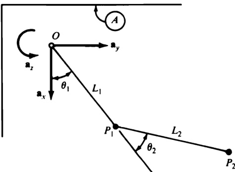
Figure P4.2

Results

\begin{array}{l}{{f_{1}={x_{1}}^{2}+{y_{1}}^{2}-{L_{1}}^{2}}}\\ {{f_{2}=(x_{2}-x_{1})^{2}+(y_{2}-y_{1})^{2}-{L_{2}}^{2}}}\\ {{f_{3}=z_{1}\qquad f_{4}=z_{2}}}\end{array}

4.3 Figure P4.3 shows two particles, \boldsymbol{P}_{1} and \pmb{P}_{2} , supported by a linkage in such a way that the position vectors, \mathfrak{p}_{1} and \pmb{{\mathbb P}}_{2} ,of \boldsymbol{P}_{1} and \scriptstyle P_{2} relative to a point o fixed in a reference frame \pmb{A} are at all times perpendicular to {\bf a}_{z} ; one of three mutually perpendicular unit vectors \mathbf{a}_{x},\mathbf{a}_{y},\mathbf{a}_{z} , fixed in \pmb{A} Determine the number of holonomic constraint equations governing motions of \boldsymbol{P}_{1} and \scriptstyle P_{2} in \pmb{A}

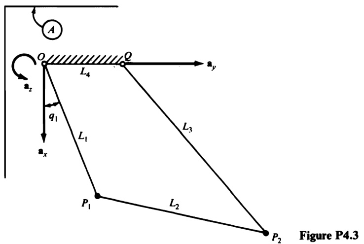
Result 5

4.4 Referring to Problem 4.1, and assuming that \boldsymbol{\theta}_{1},\,\boldsymbol{\theta}_{2} , and \theta_{3} are prescribed functions of time, show that only one generalized coordinate is required to specify the configuration of \pmb{P} in \pmb{A} , and verify that \pmb q is such a generalized coordinate.

4.5 Referring to Problem 4.2, suppose that \pmb q_{1} and \pmb q_{2} are introduced by expressing x_{i},y_{i} and z_{i}\,(i=1,2) as

\begin{array}{r l}&{x_{1}=q_{1}\qquad y_{1}=({L_{1}}^{2}-{q_{1}}^{2})^{1/2}\qquad z_{1}=0}\\ {x_{2}=q_{2}\qquad y_{2}=({L_{1}}^{2}-{q_{1}}^{2})^{1/2}+[{L_{2}}^{2}-(q_{2}-q_{1})^{2}]^{1/2}\qquad z_{2}=0}\end{array}

Verify that the four holonomic constraint equations considered in Problem 4.2 then are satisfied. Explain the following statement: “For motions during which y_{1} and y_{2} acquire negative values, \pmb q_{1} and \pmb q_{2} are not generalized coordinates." Finally, letting \pmb{\theta}_{1} and \boldsymbol{\theta}_{2} be the radianmeasures of two angles as indicatedin Fig. P4.2, show that {\bf{\nabla}}^{\theta_{1}} and \boldsymbol{\theta}_{2} are generalized coordinates for \boldsymbol{P_{1}} and \scriptstyle P_{2} in \pmb{A}

4.6 Referring to Problem 4.3, let

x_{i}\triangleq\mathbf{p}_{i}\cdot\mathbf{a}_{x}\qquad y_{i}\triangleq\mathbf{p}_{i}\cdot\mathbf{a}_{y}\qquad z_{i}\triangleq\mathbf{p}_{i}\cdot\mathbf{a}_{z}\qquad(i=1,2)

and, after noting that a single generalized coordinate suffices to characterize the configurationof \boldsymbol{P}_{1} and P_{2} in \pmb{A} attempttoexpress x_{i},\,y_{i} , and z_{i}\;(i=1,2) as functions of the angle \pmb q_{1} shown in Fig. P4.3 in such a way that all holonomic constraint equations are satisfied. Next, after expressing x_{1},y_{1} , and z_{1} as

x_{1}=L_{1}\mathbf{c}_{1}\qquad y_{1}=L_{1}\mathbf{s}_{1}\qquad z_{1}=0

and x_{2},y_{2} , and \scriptstyle z_{2} as

x_{2}=L_{1}{\bf c}_{1}+L_{2}{\bf c}_{2}\qquad y_{2}=L_{1}{\bf s}_{1}+L_{2}{\bf s}_{2}\qquad z_{2}=0

and as

x_{2}=L_{3}{\bf c}_{3}\qquad y_{2}=L_{3}{\bf s}_{3}+L_{4}\qquad z_{2}=0

show that in both cases all holonomic constraint equations are satisfied provided that q_{1},q_{2} ,and \boldsymbol{q}_{3} satisfy the two equations

\begin{array}{r}{L_{1}\mathbf{c}_{1}+L_{2}\mathbf{c}_{2}-L_{3}\mathbf{c}_{3}=0}\\ {\qquad\qquad\qquad\qquad L_{1}\mathbf{s}_{1}+L_{2}\mathbf{s}_{2}-L_{3}\mathbf{s}_{3}-L_{4}=0}\end{array}

Give a geometric interpretation of q_{2} and q_{3} , and explain the following statement: "Any one of q_{1},q_{2} , and \pmb q_{3} , but no more than one at a time, can be a generalized coordinate for P_{1} and P_{2} in \pmb{A} ”.

4.7 Determine the number of generalized coordinates of each of the following systems in a reference frame A\colon(a) Two rigid bodies attached to each other by means of a ball-and-socket joint, but otherwise free to move in A. (b) A rigid body \textbf{\emph{B}} carrying a rotor that is free to rotate relative to \pmb{B} about an axis fixed in \pmb{B} while \pmb{B} is free to move in A.\left(c\right)\mathbf{\mathrm{A}} rigid body \pmb{B} carrying a rotor that is made to rotate relative to \pmb{A} at a prescribed, time-dependent rate while \pmb{B} is free to move in A.\,(d) The system of two particles in Problem 4.2. (e) The system of two particles in Problem 4.3.

Results (a)\,9;(b)\,7;(c)\,6;(d)\,2;(e)\,1

4.8 When the disk c of Problem 2.7 moves subject to the configuration constraint that c must remain in contact with \pmb{H} then q_{1},\ldots,q_{5} are generalized coordinates for c in A . Show that u_{1},\ldots,u_{5} , defined as

u_{i}\triangleq\pmb{\mathscr{A}}_{\pmb{\mathscr{0}}}^{C}\cdot\pmb{\mathfrak{b}}_{i}\quad(i=1,2,3)\qquad u_{4}=\pmb{\mathscr{A}}_{\pmb{\mathscr{v}}}^{P}\cdot\pmb{\mathfrak{a}}_{x}\qquad u_{5}=\pmb{\mathscr{A}}_{\pmb{\mathscr{v}}}^{P}\cdot\pmb{\mathfrak{a}}_{y}

are generalized speeds for c in A , provided that |q_{2}|\neq\pi/2 rad.

4.9 Referring to Problem 2.9, and defining generalized speeds \boldsymbol{u}_{1} u_{2} ， u_{3} as (a)\,u_{i}\triangleq\,^{N}\!\mathbf{\omega}\mathbf{\omega}^{B}\cdot\mathbf{b}_{i} (i=1,2,3) and (b)\ u_{i}\triangleq{\vartriangle}^{A}{\vartriangle}_{{\bf0}}{\vline}^{B}\cdot{\vline}_{{\bf0}_{i}} (i=1,2,3) ,determine Z_{1} Z_{2} Z_{3} such that Eqs. (2.12.1) are satisfied.

Results

\begin{array}{r l}{(a)}&{Z_{1}=-\Omega\mathbf{c}_{1}\mathbf{s}_{2}}\\ &{Z_{2}=\Omega(\mathbf{c}_{1}\mathbf{c}_{2}\mathbf{s}_{3}+\mathbf{c}_{3}\mathbf{s}_{1})}\\ &{Z_{3}=\Omega(\mathbf{c}_{1}\mathbf{c}_{2}\mathbf{c}_{3}-\mathbf{s}_{3}\mathbf{s}_{1})}\\ {(b)}&{Z_{1}=Z_{2}=Z_{3}=0}\end{array}

4.10 Referring to Problem 2.7, and considering only motions of rolling of C on H, let u_{1},\dotsc,u_{5} be generalized speeds defined as in Problem 4.8. Determine A_{r s} and B_{r} (r=4,5;s=1,2,3) such that Eqs. (2.13.1) are satisfied.

Results

\begin{array}{r l r l r l r}&{A_{41}=0}&&{A_{42}=R\cos q_{1}\tan q_{2}}&&{A_{43}=-R\cos q_{1}}\\ &{A_{51}=0}&&{A_{52}=R\sin q_{1}\tan q_{2}}&&{A_{53}=-R\sin q_{1}}\\ &{B_{4}=B_{5}=0}&&{}\end{array}

4.11 Figure P4.11 shows two sharp-edged circular disks, C_{1} and C_{2} , each of radius R , mounted at the extremities of a cylindrical shaft s of length 2L , the axis of S coinciding with those of C_{1} and C_{2} . The disks are supported by a plane P that is fixed in a reference frame A ,and they can rotate freely relative to \boldsymbol{S}

Six generalized speeds suffice to characterize all motions of C_{\mathrm{i}} C_{2} ,and _{\textrm{\scriptsize{\it{S}}}} in A. Defining these as

{\begin{array}{r l r l r}&{u_{1}\triangleq^{A}\mathbf{v}^{S^{\ast}}\cdot\mathbf{n}_{1}}&&{u_{2}\triangleq^{A}\mathbf{\omega}^{S}\cdot\mathbf{n}_{2}}&&{u_{3}\triangleq^{A}\mathbf{\omega}^{S}\cdot\mathbf{n}_{3}}\\ &{u_{4}\triangleq^{A}\mathbf{\omega}^{C_{1}}\cdot\mathbf{n}_{3}}&&{u_{5}\triangleq^{A}\mathbf{\omega}^{C_{2}}\cdot\mathbf{n}_{3}}&&{u_{6}\triangleq^{A}\mathbf{v}^{S^{\ast}}\cdot\mathbf{n}_{3}}\end{array}}

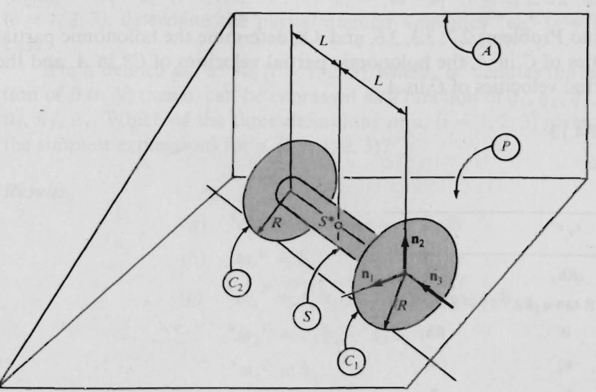
where \mathbf{n}_{1},\,\mathbf{n}_{2} , and \mathbb{n}_{3} are mutually perpendicular unit vectors, with \mathbb{n}_{2} normal to \pmb{P}_{\cdot} , as shown in Fig. P4.11, and s^{*} is the mass center of S, show that when C_{1} and C_{2} roll on P , then u_{4},\,u_{5} , and \pmb{u}_{6} each can be expressed in terms of u_{1},u_{2} , and \pmb{u}_{3} by means of an equation having the form of Eq. (2.13.1). Determine A_{r s} and B_{\nu} \overset{\cdot}{r},(r=4,5,6;s=1,2,3)

Results

\begin{array}{l c r}{{A_{41}=\,-1/R\,}}&{{A_{42}=L/R\,}}&{{A_{43}=0}}\\ {{A_{51}=\,-1/R\,}}&{{A_{52}=\,-L/R\,}}&{{A_{53}=0}}\\ {{A_{61}=A_{62}=A_{63}=0}}&{{}}&{{}}\\ {{B_{4}=B_{5}=B_{6}=0}}&{{}}&{{}}\end{array}

4.12/ Referring to Problem 4.11, suppose that motors connecting s to C_{1} and C_{2} areused to cause C_{1} and C_{2} to rotate in such a way that

{\}^{s}{\pmb{\upomega}}^{C_{1}}=\Omega_{1}{\pmb{\up n}}_{3}\qquad{\}{\pmb{\upomega}}^{C_{2}}=\Omega_{2}\,{\pmb{\up n}}_{3}

where \Omega_{1} and \Omega_{2} are prescribed functions of the time t. Show that the system formed by S, C_{1} and C_{2} possesses one degree of freedom in \pmb{A} if C_{1} and C_{2} roll on \pmb{A} ,and determine A_{r1} and B_{r}\;(r=2,\ldots,6) such that u_{2},\ldots,u_{6} satisfy Eqs. (2.13.1).

Results

\begin{array}{r l r l}&{A_{21}=0}&&{B_{2}=\frac{1}{2}(R/L)(\Omega_{1}-\Omega_{2})}\\ &{A_{31}=-1/R}&&{B_{3}=-\frac{1}{2}(\Omega_{1}+\Omega_{2})}\\ &{A_{41}=-1/R}&&{B_{4}=\frac{1}{2}(\Omega_{1}-\Omega_{2})}\\ &{A_{51}=-1/R}&&{B_{5}=\frac{1}{2}(\Omega_{2}-\Omega_{1})}\\ &{A_{61}=0}&&{B_{6}=0}\end{array}

4.13 Referring to Problems 2.7, 3.3, 3.6, and 4.8, determine the holonomic partial angular velocities of c in \pmb{A} , the holonomic partial velocities of C^{*} in \pmb{A} , and the holonomic partial velocities of \hat{C} in \pmb{A}

Results Table P4.13

Table P4.13

<html>

r	A0,C	Av,c"	Av,c
1	b1	Rb3	0
2	b2	-R tan q2b	-R tan q2b1
3	b3	0	Rb1
4	0	ax	ax
5	0	ay	ay

</html>

4.14With u_{1},\dots,u_{5} defined as in Problem 4.8, and considering only motions of roHing of c on \pmb{H} , determine the nonholonomic partial angular velocities of c in A , the nonholonomic partial velocities of C^{*} in \pmb{A} , and the nonholonomic partial velocities of \hat{C} in \pmb{A} . Do this by inspecting expressions for ^{A}\!{\boldsymbol{\omega}}^{c},{^{A}\!{\bf{v}}^{c}}, and \pmb{A}_{\mathbf{v}}\bar{\pmb{c}} then check the results by using Eqs. (2.14.15) and (2.14.17) in conjunction with information available in Problems 4.10 and 4.13.

Results Table P4.14

Table P4.14

<html>

r	Ao,C		AvC
1	b1	Rb3	0
2	b2	0	0
3	b3	-Rb1	0

</html>

*_{\mathbf{4.15}} The configuration of a system S in a reference frame \pmb{A} is characterized by generalized coordinates q_{1},\ldots,q_{n} . Taking u_{r}\triangleq{\dot{q}}_{r}\ (r=1,\dots,n), , and letting \pmb{\upbeta} be a vector fixed in a rigid body \boldsymbol{B} belonging to S, show that

\frac{^{A}\partial\mathfrak{B}}{\partial q_{r}}=\mathfrak{w}_{r}\times\mathfrak{B}\qquad(r=1,\,.\,.\,.\,,n)

where \mathbf{o}_{r} is the rth partial angular velocity of \pmb{B} in \pmb{A}

4.16 Referring to Problem 2.9, and defining generalized speeds u_{1},u_{2},\ u_{3} as (a)\cup_{i}={}^{N}\!\mathbf{\omega}\mathbf{\omega}^{B}\cdot\mathbf{b}_{i} (i=1,2,3) , (b) u_{i}\triangleq\mathbf{\omega}_{\mathbf{0}}^{A}\mathbf{\omega}^{B}\cdot\mathbf{b}_{i} (i=1,2,3) ,and (c) u_{i}=\dot{q}_{i} (i=1,2,3) , determine the partial angular velocities ^N\mathbf{\omega}_{\mathbf{0}_{r}}^{B}\ (r=1,\ 2,\ 3) in each case.

If \alpha_{i} is defined as {}^{N}\!\mathfrak{d}^{B}\cdot\mathfrak{b}_{i}\left(i=1,2,3\right) ,where \pmb{N}_{\pmb{\alpha}}\pmb{B} denotes the angular acceleration of \pmb{B} in N , then \pmb{\alpha}_{i} can be expressed as a function of q_{1},q_{2},q_{3},u_{1},u_{2},u_{3} , and \dot{u}_{1},\,\dot{u}_{2},\,\dot{u}_{3} . Which of the three definitions of u_{i} \mathbf{\Phi}_{i}\left(i=1,2,3\right) given above leads to the simplest expressions for \alpha_{i}\,(i=1,2,3)

Results

\begin{array}{r l}{(a)}&{^{N}\mathbf{0}_{r}^{\phantom{\,}_{B}\,}=\mathbf{b}_{r}\qquad(r=1,2,3)}\\ {(b)}&{^{N}\mathbf{0}_{r}^{\phantom{\,}_{B}\,}=\mathbf{b}_{r}\qquad(r=1,2,3)}\\ {(c)}&{^{N}\mathbf{0}_{1}^{\phantom{\,}_{B}\,}=\mathbf{c}_{2}\mathbf{b}_{1}+\mathbf{s}_{2}\mathbf{s}_{3}\mathbf{b}_{2}+\mathbf{s}_{2}\mathbf{c}_{3}\mathbf{b}_{3}}\\ &{^{N}\mathbf{0}_{2}^{\phantom{\,}_{B}\,}=\mathbf{c}_{3}\mathbf{b}_{2}-\mathbf{s}_{3}\mathbf{b}_{3}}\\ &{^{N}\mathbf{0}_{3}^{\phantom{\,}_{B}\,}=\mathbf{b}_{1}}\end{array}

Definition (a) leads to the simplest expression for \alpha_{i}\,(i=1,2,3)

\ast4.17 Referring to Problem 3.15, determine the partial angular velocities \varepsilon_{\pmb{\omega}_{r}}\pmb{A} \varepsilon_{\mathbf{\upomega}_{r}^{B},\mathbf{\xi}^{E}\mathbf{\omega}_{\mathbf{\upomega}_{r}}^{C}} , and \varepsilon_{\pmb{\omega}_{r}}\pmb{D} (r=1,2,3) and the partial velocities \mathbf{\bar{\boldsymbol{\varepsilon}}_{v_{r}}}^{A^{*}},\mathbf{\boldsymbol{\varepsilon}_{v_{r}}}^{B^{*}},\mathbf{\boldsymbol{\varepsilon}_{v_{r}}}^{C^{*}} and \varepsilon_{\mathbf{v}_{r}}^{{\scriptscriptstyle{D}}*}(r=1,2,3)

Results Tables P4.17(a), P4.17(b)

Table P4.17(a)

<html>

	EW,A	EO,B	E@,C	EW,D
	a1	c,b, + s,b3	c,b1+ sb3	cb1 + sb3
2	0	b2	b2	b2
3	0	0	0	0

</html>

Table P4.17(b)

<html>

		Ev
1	-LAa2	Z6b2	Z10b2	Z13b1 + Z1sb2 + Z16b3
2	0	Lgb1	Z,b1	Z14b1-Pb3
3	0	0	b3	b3

</html>

4.18 In Problem 4.8, five generalized speeds are defined for c in \pmb{A} An alternative set of generalized speeds can be introduced by defining u_{1},\ldots,u_{5} as

u_{r}\triangleq{\dot{q}}_{r}\qquad(r=1,\dots,5)

When ^{c} rolls on \pmb{H} , these generalized speeds satisfy constraint equations of the form of Eqs. (2.13.1), with A_{43}=-R cos \boldsymbol{q}_{1} A_{53}=-R sin \pmb q_{1} and A_{r s}=B_{r}=0 for r=4. 5 and s=1 , 2. Furthermore, the velocity of C^{*} in \pmb{A} is given by

^{A}\mathbf{v}^{C^{*}}=\,-\,R[(u_{1}\,\sin\,q_{2}\,+\,u_{3})\mathbf{b}_{1}\,+\,u_{2}\,\mathbf{b}_{3}]

To verify that it can be far more laborious to work with the right-hand members of Eqs. (2.15.7) than with the left-hand members, determine A_{\widetilde{\Psi}_{r}}c^{*}\cdot A_{{\mathbf{a}}}c^{*}(r=1,2,3) where \mathbf{\Psi_{a}}\mathbf{c}^{*} is the acceleration of c^{*} in \pmb{A} by (a) forming s_{\widetilde{\mathbf{v}}_{r}}c^{*} by inspection of the expression given above for \pmb{A}_{\mathbf{v}}\pmb{c}^{\star} forming \mathbf{\Psi_{a}}\mathbf{c}^{\bullet} by differentiating \pmb{A}_{\mathbf{v}}\pmb{c}\bullet with respect to time t in \pmb{A} , and then dot-multiplying \mathbf{\mathcal{A}}_{\widetilde{\mathbf{V}}}\mathbf{\mathcal{C}}^{*} with {^{A}\mathfrak{a}^{C^{\ast}}}\left(r=1,\bar{2},3\right) and (b) using the right-hand members of Eqs. (2.15.7).

Results

{^{A}\tilde{\mathbf{v}}_{1}}^{\scriptscriptstyle C^{*}}\cdot{^{A}\mathbf{a}}^{C^{*}}=R^{2}(\dot{u}_{1}\sin q_{2}+2u_{1}u_{2}\cos q_{2}+\dot{u}_{3})\sin

\begin{array}{r l}&{^{\alpha}\mathbf{v}_{1}^{\phantom{*}}\cdot\mathbf{\nabla}^{*}\mathbf{a}^{*}\ =\,K^{*}(u_{1}\ \mathrm{sin}\ q_{2}+2u_{1}u_{2}\cos q_{2}+u_{3})\,\mathrm{s}}\\ &{^{\cal A}\tilde{\mathbf{v}}_{2}^{\phantom{*}}\cdot{\cal A}\mathbf{a}^{C^{*}}=\,R^{2}[\dot{u}_{2}\ -{\cal u}_{1}\cos q_{2}(u_{1}\ \mathrm{sin}\ q_{2}+u_{3})]\,}\\ &{^{\cal A}\tilde{\mathbf{v}}_{3}^{\phantom{*}}\mathrm{c}^{*}\cdot{\cal A}\mathbf{a}^{C^{*}}=\,R^{2}(\dot{u}_{1}\ \mathrm{sin}\ q_{2}+2u_{1}u_{2}\ \mathrm{cos}\ q_{2}+\dot{u}_{3})\,}\end{array}

PROBLEM SET 5

(Secs. 3.1-3.5)

5.1 Regarding Fig. P5.1 as showing two views of a body \pmb{B} formed by matter distributed uniformly (a) over a surface having no planar portions and (b) throughout a solid, determine (by integration) the coordinates x^{*},\,y^{*},\,z^{*} of the mass center of \pmb{B}

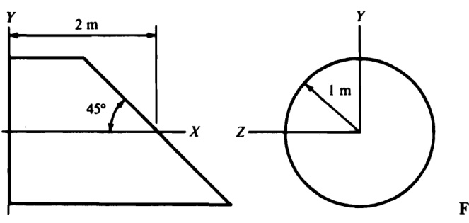
Figure P5.1

Results Table P5.1

Table P5.1

<html>

x* (m)	y* (u)	2* (u)
(a) 001o	-t	0
(b)	1	一 0

</html>

5.2 Regarding Fig. P5.2 as showing two views of a body \pmb{B} formed by matter distributed uniformly (a) over a surface having no planar portions and (b) throughout a solid, determine (without integration) the X -coordinate of the mass center of \pmb{B}

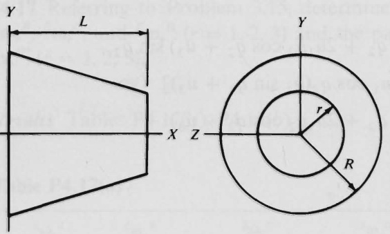
FigureP5.2

(a)\ \frac{L}{3}\frac{R\,+\,2r}{R\,+\,r}\quad(b)\ \frac{L}{4}\frac{R^{2}\,+\,2r R\,+\,3r^{2}}{R^{2}\,+\,r R\,+\,r^{2}}

\ast\mathbf{5.3} Prove the following theorems (known as “theorems of Pappus" or "Guldin's rules"):

When a plane curve C of length L is revolved about a line lying in the plane of C and not intersecting C , the area of the surface of revolution thus generated is equal to theproduct of L and the circumference of the circle described by the centroid of C

When a plane region R of area A is revolved about a line lying in the plane of R and not passing through R , the volume of the solid of revolution thus generated is equal to the product of A and the circumference of the circle described by the centroid of R

Use these theorems to locate the centroids of a semicircular curve and a semicircular sector,keeping in mind that the surface area and the volume of a sphereofradius R areequal to 4\pi R^{2} and 4\pi R^{3}/3 respectively.

5.4Parts A,B,C,D of the assembly shown in Fig. P5.4 are made of steel (7800 {\bf k g}/{\bf m}^{3}) ,sheetmetal (17.00\,\mathrm{kg/m}^{2}) ,aluminum (2700\,\mathrm{kg}/\mathrm{m}^{3}) ),andbrass (8400\,\mathrm{kg/m}^{3})

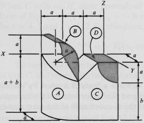
FigureP5.4

respectively. (a) For a=b=0.3\mathrm{~m} , determine the coordinates x^{*},y^{*},z^{*} of the mass center of the assembly. (b) For a=0.3\;\mathrm{m} determine to three significant figures the range of values of \pmb{b} such that x^{*}=0.400

(a)\,0.434\mathrm{\,m,}0.135\mathrm{\,m,}-0.300\mathrm{\,m}\quad(b)\,0.136\mathrm{\,m}\leq b\leq0.138\mathrm{\,m}
$$Results  

5.5 Show by means of an example that ${\bf I}_{a}$ as defined in Eq. (3.3.1) can be, but need not be, parallel to $\mathbb{n}_{a}$  

5.6 Unit vectors $\mathbf{n}_{\mathbf{x}},\,\mathbf{n}_{\mathbf{y}}$ , and $\pmb{\mathrm{\scriptscriptstyle{u}}}_{\pmb{z}}$ are respectively parallel to the axes OX, OY, OZ of a rectangular Cartesian coordinate system, and each unit vector points in the positive direction of the axis to which it is parallel. Letting S be a set of $\pmb{\nu}$ particles, $m_{i}$ the mass of particle $\boldsymbol{P}_{i}$ , and $x_{i},y_{i}$ , and $z_{i}$ the coordinates of $\boldsymbol{P}_{i}$ $\mathit{\Omega}(i=1,\dots,\nu)$ express $I_{x}$ , the moment of inertia of $\boldsymbol{s}$ about the $X$ -axis, and $I_{y z}$ , the product of inertia of S relative to $o$ for $\mathbf{n_{y}}$ and $\pmb{\mathrm{\scriptscriptstyle{R}}}_{\pmb{\mathrm{\scriptscriptstyle{z}}}}$ , in terms of the masses and coordinates of $P_{1};...,P_{\nu}$ . Then answer the following questions: $(a)$ Does it matter whether $\mathbf{n}_{\mathbf{x}},\mathbf{n}_{\mathbf{y}}$ , and $\pmb{\mathrm{~m~}}_{\pmb{z}}$ form a right-handed or a left-handed set of unit vectors? $(b)$ Would the results be altered if $O X,O Y,$ and $_{o Z}$ were not mutually perpendicular?  

I_{x}=\sum_{i=1}^{\nu}m_{i}({y_{i}}^{2}+,{z_{i}}^{2})\qquad I_{y z}=,-\sum_{i,=,1}^{\nu}m_{i}y_{i}z_{i}\qquad(a),\mathrm{No}\qquad(b),\mathrm{Yes}

  

5.7 Show by means of examples that products of inertia can be positive, negative, or zero, and that radii of gyration can be equal to zero.  

$\bf{*5.8}$ A body $\pmb{B}$ of mass m is modeled as matter distributed uniformly along a helix $\pmb{H}$ constructed by drawing a straight line $L$ on a rectangular sheet of paper having the dimensions shown in Fig. P5.8 and then bending the paper to form a right-circular cylinder. Letting $\mathbb{n}_{1}$ and $\mathbb{n}_{2}$ be unit vectors directed as shown, determine ${\bf{I}}_{1}$ and ${\bf{I}}_{2}$ , the inertia vectors of $\pmb{B}$ relative to the mass center of $\pmb{B}$ for $\mathbb{n}_{1}$ and $\triangledown_{2}$ ,respectively.  

{\bf I}{1}=m a^{2}{\bf n}{1}+[m a b/(2\pi)]{\bf n}{1}\times{\bf n}{2}\qquad{\bf I}{2}=(m/2)(a^{2}+b^{2}/6){\bf n}{2}

  

![](images/cecb0108dd31db62ec42057c5989d63794d115fbbad61eb5c9226bca479da771.jpg)  

Figure P5.8  

5.9 A line $L_{a}$ passes through a point $o$ and is perpendicular to the unit vector $\mathbf{n}_{3}$ of a set of mutually perpendicular unit vectors $\mathbf{n}_{1},\mathbf{n}_{2}$ ,and $\mathbf{n}_{3}$ . Under these circumstances, $\scriptstyle{I_{a}}$ ,themomentofinertiaof abody $B$ about line $L_{a}$ ,dependson the orientation of $L_{a}$ in the plane that passes through $o$ and is perpendicular to $\mathbf{n}_{3}$  

Express the maximum and minimum values of $I_{a}$ in terms of $I_{1},I_{2}$ , and $I_{\mathrm{~1~2~}}$ the inertia scalars of $B$ relative to $o$ for ${\bf{n}}_{1}$ and $\mathbf{n}_{2}$ ,and,lettingcos $\theta\ \mathbf{n}_{1}+\sin\theta\ \mathbf{n}_{2}$ be a unit vector parallel to $L_{a}$ ,showthat  

\tan2\theta=\frac{2I_{12}}{I_{1}-I_{2}}

  

when $I_{a}$ has a maximum or minimum value.  

Result  

\frac{I_{1}+I_{2}}{2}\pm\left[\left(\frac{I_{1}-I_{2}}{2}\right)^{2}+I_{12}{}^{2}\right]^{1/2}

  

5.10 In Fig. P5.10, $\mathbf{n}_{1}$ $\mathbf{n}_{2}$ , and ${\bf\vec{n}}_{3}$ are mutually perpendicular unit vectors, and $B^{*}$ designates the mass center of a body $B_{\cdot}$ The inertia scalars of $B$ relativetopoint $o$ for $\mathbf{n}_{1},\,\mathbf{n}_{2}$ , and ${\bf\tilde{n}}_{3}$ are shown in units of ${\bf k g}\;{\bf m}^{2}$ in Table P5.10.  

Table P5.10   


<html><body><table><tr><td>1 2 3</td></tr><tr><td>1 260 72 -144</td></tr><tr><td>2 72 325 9%6</td></tr><tr><td>3 -144 96 169</td></tr></table></body></html>  

![](images/a6f6ab1dfc41f4015913bd6bdc53d879673e4d01fcd80a6a3a66bc4237ba7730.jpg)  
Figure P5.10  

Determine the moment of inertia of $B$ with respect to a line that is parallel to line $P Q$ and passes through point $o$  

Result $340\,\mathrm{kg}\;\mathrm{m}^{2}$  

5.11 Referring to Problem 5.10, and letting $\mathbf{e}_{1},\mathbf{e}_{2}$ ,and ${\bf e}_{3}$ be unit vectors defined as  

\mathbf{e}{1}\triangleq-\mathbf{n}{3}\qquad\mathbf{e}{2}\triangleq\mathbf{n}{1}\qquad\mathbf{e}{3}\triangleq\mathbf{n}{2}

  

form the inertia matrix of $B$ relative to $o$ for $\mathbf{e}_{1},\mathbf{e}_{2}$ ,and $\mathbf{e}_{3}$  

Result  

\left[{\begin{array}{r r r r}{169}&{144}&{-96}\ {144}&{260}&{72}\ {-96}&{72}&{325}\end{array}}\right]

  

$\mathbf{*5.12}$ Solve Problem 5.10 by performing multiplications of a row matrix with the matrix constructed in Problem 5.11.  

5.13 If $\mathbf{n}_{1},\,\mathbf{n}_{2},\,\mathbf{n}_{3}$ and ${\bf\bar{n}}_{1}^{\prime},{\bf\bar{n}}_{2}^{\prime},{\bf\bar{n}}_{3}^{\prime}$ are two sets of unit vectors, the unit vectors of each set are mutually perpendicular, and $C_{i j}$ is defined as  

C_{i j}\triangleq\mathfrak{n}{i}\cdot\mathfrak{n}{j}^{\prime}\qquad(i,j=1,2,3)

  

then the $3\times3$ matrix $^c$ having $C_{i j}$ as the jth element of the ith row called a direction cosine matrix for the two sets of unit vectors. Letting $C^{T}$ denote the tranispose of $c$ ,showthat $\boldsymbol{I}$ and $r$ , the inertia matrices of a set $\boldsymbol{s}$ for a point $_o$ for $\mathbf{n}_{1},\mathbf{n}_{2},\mathbf{n}_{3}$ and ${\bf\bar{n}}_{1}^{\prime},{\bf\bar{n}}_{2}^{\prime},{\bf\bar{n}}_{3}^{\prime}$ , respectively, are related to each other as follows:  

I^{\prime}=C^{\tau}I C

  

$\mathbf{*5.14}$ The time-derivative of a dyadic $\mathbf{D}$ in a reference frame $\pmb{A}$ is defined as  

\frac{A_{d\mathbf{D}}}{d t}\triangleq\sum_{i=1}^{3},\sum_{j=1}^{3}\mathbf{a}{i}\mathbf{a}{j}\frac{d}{d t}\left(\mathbf{a}{i}\cdot\mathbf{D}\cdot\mathbf{a}{j}\right)

  

where ${\bf a}_{1},{\bf a}_{2},{\bf a}_{3}$ are mutually perpendicular unit vectors fixed in $\pmb{A}.$ Show that the time-derivatives of $\mathbf{D}$ in two reference frames $\pmb{A}$ and $\pmb{B}$ are related by  

\frac{{}^{A}d\mathbf{D}}{d t}=\frac{{}^{B}d\mathbf{D}}{d t}+,\sp{A}!\mathbf{\omega}"\times\mathbf{D}-\mathbf{D},\times,\sp{A}!\mathbf{\omega}^{B}

  

where $\pmb{A}_{\pmb{\omega}}\pmb{B}$ is the angular velocity of $\pmb{B}$ in $\pmb{A}$  

# PROBLEM SET 6  

# (Secs. 3.6-3.9)  

6.1 A point $o$ of a rigid body $\pmb{B}$ is fixed in a reference frame A. Show that $\mathbf{H}_{\mathrm{:}}$ the angular momentum of $\pmb{B}$ relative to $o$ in $\pmb{A}$ , is given by Eq. (3.5.28) if I denotes the inertia dyadic of $\pmb{B}$ relative to $o$ and $\mathbf{\delta}\mathbf{o}$ is the angular velocity of $\pmb{B}$ in $\pmb{A}$  

$\ast_{\mathbf{6.2}}$ A rigid body $\textbf{\emph{B}}$ moves in a reference frame $\pmb{A}$ with an angular velocity @. Show that the central angular momentum of $\pmb{B}$ in $\pmb{A}$ is parallel to $\mathbf{\delta}\mathbf{o}$ if and only if $\mathbf{\delta}_{\mathbf{\delta}}^{\mathbf{\delta}}$ is parallel to a central principal axis of $\pmb{B}$  

6.3 Letting $\mathbf{H}^{s/o}$ ， $\mathbf{H}^{s/s^{*}}$ and $\mathbf{H}^{\mathbf{S}\ast_{I}\boldsymbol{o}}$ denote, respectively, the angular momentum of a set S of particles relative to a point $o$ in a reference frame $\pmb{A}$ , the central angular momentum of $s$ in $\pmb{A}$ , and the angular momentum in $\pmb{A}$ , relative to $^o$ , of a particle whose motion is identical to that of the mass center $s^{*}$ of $\boldsymbol{s}$ and whose mass is equal to the total mass of S, show that  

\mathbf{H}^{s/o}=\mathbf{H}^{s/S^{}}+\mathbf{H}^{s/O}

  

$\clubsuit\ensuremath{\mathbf{6.4}}$ Letting ${}^{E}\!{\bf H}^{C/C*},{}^{E}\!{\bf H}^{D/C*}$ and $^{\mathbf{\deltaA}}\mathbf{H}^{\mathbf{\alphaB/c^{*}}}$ denote angular momenta, show that  

\begin{array}{r}{{^{E}!{\bf H}^{C/C*}}={^{E}!{\bf H}^{D/C*}}+{^{A}!{\bf H}^{B/C*}}}\end{array}

  

ü $A,B,C,D,E,$ and $C^{*}$ are defined as follows: $\pmb{A}$ a rigid body; $B;$ a set of particles; $c$ , the system formed by $\pmb{A}$ and $B;D_{\mathrm{:}}$ a rigid body that has the same motion as $\pmb{A}$ and the same mass distribution as $C;E_{\mathrm{:}}$ a reference frame; $c^{*}$ , the mass center of $c$  

$\bf{*}_{6.5}$ The mass center of a rigid body $\pmb{B}$ is fixed in a rigid body $\pmb{A}$ ,but $\pmb{B}$ is otherwise free to move relative to $\pmb{A}$ Letting $c$ be the system formed by $\pmb{A}$ and $\pmb{B}$ , show that $\mathbf{H},$ the central angular momentum of $c$ in a reference frame $E_{\cdot}$ , is given by  

\mathbf{H}=\mathbf{I}{B}\cdot{}^{A}\mathbf{\omega}\mathbf{\omega}^{B}+\mathbf{I}{C}\cdot{}^{E}\mathbf{\omega}^{A}

  

where ${\bf{I}}_{\pmb{B}}$ and $\mathbf{I}_{c}$ are the central inertia dyadics of $\pmb{B}$ and $c$ ,respectively, while $\mathbf{\hat{\omega}_{G D}}^{B}$ and $\pmb{\varepsilon_{\pmb{\upomega}}}_{\pmb{\upomega}}\pmb{A}$ are the angular velocities of $\pmb{B}$ in $\pmb{A}$ and $\pmb{A}$ in ${\pmb E}$ , respectively.  

6.6Thebody $\pmb{B}$ of Problem 5.10 has a mass of $12\;\mathbf{kg}$ Determine themoment of inertia of $\pmb{B}$ about line $P Q$ , and find the product of inertia of $\pmb{B}$ relative to $B^{*}$ for $\mathbf{\overline{{u}}_{1}}$ and $\mathbb{n}_{2}$ ：  

Results $3316/25\,\mathrm{{kg\,m^{2}}};$ 0  

6.7 Three identical uniform, square plates, each of mass $m$ , are attached to each other as shown in Fig. P6.7. Determine the value of $\theta$ for which the radius of gyration of this assembly with respect to line $L$ has a minimum value, and find this value.  

Results 340°; 0.696b  

![](images/84b637696b226860326c1920472c8d6ce168088e90e72a1273537f77be809d95.jpg)  
Figure P6.7  

$\mathbf{6.8\,\textbf{A}}$ thin-walled, right-circular, cylindrical shell has a radius $R$ andheight $H$ Determine the radius of gyration of the shell with respect to a line that passes through the mass center and is perpendicular to the axis of the shell.  

Result $(R^{2}/2\,+\,H^{2}/12)^{1/2}$  

6.9 Verify each of the following statements and provide an illustrative example: $(a)$ A central principal axis of a body is a principal axis for each point of the axis. $(b)$ If a principal axisfor a point other than the mass center passes through the mass center,it is a central principal axis. (c) A line that is a principal axis for two of its points is a central principal axis. $(d)$ The three principal axes for a point on a central principal axis are parallel to central principal axes. (e) If two principal moments of inertia for a given point are equal to each other, then the moments of inertia with respect to all lines passing through this point and lying in the plane determined by the associated principal axes are equal to each other. $(f)$ If the particles of a set $s$ lie in aplane $P$ thentheline $L$ normalto $P$ and intersecting $P$ at a point $o$ is a principal axis of $s$ for $o$ ,and the moment of inertia of $s$ about $L$ is equal to the sum of the moments of inertia of $s$ about any two orthogonal lines that lie in $P$ and intersect at $o$  

6.10 Determine the smallest angle between line $A B$ and any principal axis for point $\boldsymbol{A}$ of the thin, uniform, rectangular plate represented by the shaded portion ofFig.P6.10.  

![](images/ffe65c0c86b13fd30ed92c751342ebe6350a2b58b31bb1a573536bd5ce43d368.jpg)  
Figure P6.10  

6.11 For $I_{j k}$ $j,k=1,2,3)$ as in Eq. (3.5.22), show that no one of $I_{j j}\,(j=1,2,3)$ can exceed the sum of the other two, and that $-I_{11}/2\leq I_{23}\leq I_{11}/2,$ $-I_{22}/2\leq$ $I_{31}\leq I_{22}/2$ ,and $-I_{33}/2\leq I_{12}\leq I_{33}/2$  

$\ast_{6.12}$ Defining $C_{1},C_{2}$ , and $C_{3}$ as  

\begin{array}{r l}&{C_{1}\triangleq I_{1}+I_{2}+I_{3}}\ &{C_{2}\triangleq I_{1}I_{2}+I_{2}I_{3}+I_{3}I_{1}-{I_{12}}^{2}-{I_{23}}^{2}-{I_{31}}^{2}}\ &{C_{3}\triangleq I_{1}I_{2}I_{3}+2I_{12}I_{23}I_{31}-{I_{1}}{I_{23}}^{2}-{I_{2}}{I_{31}}^{2}-{I_{3}}{I_{12}}^{2}}\end{array}

  

where $I_{j}\triangleq I_{j j}$ and $I_{j k}$ is the inertia scalar of a set of particles relative to a point for unit vectors $\mathbf{n}_{j}$ and ${\bf n}_{k}\left(j,k=1,2,3\right)$ , show that the values of $C_{1},C_{2}$ , and $C_{3}$ are independent of the way $\mathbf{n}_{1},\,\mathbf{n}_{2}$ , and $\mathbf{n}_{3}$ are chosen, so long as these vectors are mutuallyperpendicular.  

Suggestion: Verify that Eq. (3.8.7) can be written  

{I_{z}}^{3}\mathrm{-}{C_{1}}{I_{z}}^{2}\mathrm{+}{C_{2}}{I_{z}}\mathrm{-}{C_{3}}=0

  

6.13 Four identical particles are placed at the points $O,\,P,\,Q,\,R$ of Fig.P5.10. Determine the minimum radius of gyration of this set of particles, and find the smallest angle between the associated principal axis and line $O P$  

Results 1.436 m, 67.64°  

6.14 Twoidentical, thin,uniform, right-triangular plates are attached to each other as shown in Fig. P6.14. When $a/b$ is given, $k$ the minimum radius of gyration of this assembly, can be expressed as $k=n b$ Determine $n$ for $a/b=2$ and $a/b=0.5$  

![](images/56f59cfd90c5135dbcec04b9e0a8173d1c2bdb8e5eaeab07f804913d1ab5d490.jpg)  
Figure P6.14  

Results ${}\quad{\frac{1}{3}},$ $.\,[35-(241)^{1/2}]^{1/2}/24$  

$^{*}6.15$ Letting $E$ be an inertia ellipsoid of a set $s$ of particles for a point $o$ ,and letting $R$ be the distance from $o$ to a point $P$ on the surface of $E$ ,show that ${\bf I}_{a}$ the inertia vector of $s$ relative to $o$ for ${\bf{n}}_{a}$ , a unit vector directed from $o$ to $P$ ,is perpendicularto $E$ at $P$  

Note:If $\mathbf{n}_{x},\mathbf{n}_{y},\mathbf{n}_{z}$ are mutually perpendicular unit vectors,the position vector ${\bf r}^{o P}$ fromapoint $o$ toa point $P$ of a surface $\sigma$ is expressed as  

{\bf r}^{O P}=x{\bf n}{x}+y{\bf n}{y}+z{\bf n}_{z}

  

and the equation of $\sigma$ is written $f(x,y,z)=0$ then $\mathbf{\nabla}\mathbf{V}f$ a vector defined as  

\nabla f\triangleq{\frac{\partial f}{\partial x}},\mathbf{n}{x}+{\frac{\partial f}{\partial y}},\mathbf{n}{y}+{\frac{\partial f}{\partial z}},\mathbf{n}_{z}

  

and called the gradient of $f,$ is perpendicular to $\sigma$ at $P$  

$\bf{*}6.16$ For a set $s$ of particles $P_{1},\dots,P_{\nu}$ moving in a reference frame $A$ a quantity $G$ ,known as a Gibbs function for $s$ in $A$ ,is defined as  

G\triangleq{\frac{1}{2}}\sum_{i=1}^{\nu}m_{i}{\mathbf{a}_{i}}^{2}

  

where $m_{i}$ and $\mathbf{a}_{i}$ are the mass of ${\mathbf{}}P_{i}$ and the acceleration of ${\mathbf{}}P_{i}$ in $A$ ,respectively.  

Letting $B$ be a rigid body, express the Gibbs function for $B$ in $A$ in terms of the acceleration a of the mass center of $\boldsymbol{B}$ in $A$ ,the angular velocity $\mathbf{\omega}$ of $B$ in $A$ the angular acceleration $\pmb{\upalpha}$ of $B$ in $A$ , the mass $m$ of $\boldsymbol{B}$ and the central inertia dyadic I of $B$  

\begin{array}{r}{G=\frac{1}{2}(m\mathbf{a}^{2}+\alpha\cdot\mathbf{I}\cdot\alpha+2\alpha\cdot\omega\times\mathbf{I}\cdot\mathbf{\omega}+\mathbf{\omega}\mathbf{\omega}^{2}\mathbf{\omega}\cdot\mathbf{I}\cdot\mathbf{\omega})}\end{array}

  

# PROBLEM SET 7  

# (Secs. 4.1-4.3)  

7.1 Two forces, A and B, of equal magnitude act along the lines $P Q$ and $\pmb{R S}$ in Fig. P7.1 and are directed as there indicated. Determine the angle $9(0\leq\theta\leq180^{\circ})$ between the resultant of this force system and the moment of the force system aboutpoint $^o$  

Result $117.12^{\circ}$  

![](images/6906d5b8ebea72a37c7d7d525a69ecbbd84983220b5af2afff5b0c44d83aa819.jpg)  

Figure P7.1  

7.2 Referring to Problem 7.1, let A and $\mathbf{\deltaB}$ each have a magnitude of $10~\mathrm{\bfN}$ and let C be a force applied at point $^o$ in such a way that A, B, and C form a couple. Determine the magnitude of the torque of this couple.  

# Result 90.56 N m  

7.3 Show by means of an example that there exist sets of bound vectors such that the moment of the set of vectors about a point differs from the moment of the resultant about that point, no matter where the resultant is applied.  

7.4 Show that the moments of a set $\boldsymbol{s}$ of bound vectors about all points of any line parallel to the resultant of S are equal to each other.  

7.5 Letting M be the moment about a point $o$ of a set S of bound vectors, and resolving M into two components, one parallel to $\mathbf{R}$ , the resultant of S, the other perpendicular to $\mathbf{R}_{}$ . show that the magnitude of the first of these is independent of thelocation of $^o$  

7.6 If a set S of bound vectors is not a couple, the points about which S has a moment $\mathbf{M}^{*}$ of minimum magnitude lie on a line $L^{*}$ that is parallel to $\pmb{\mathrm{R}}_{\mathrm{:}}$ the resultantof $s.L^{*}$ is called the central axis of S.  

Letting M be the moment of $\boldsymbol{s}$ about a reference point $^o$ selected arbitrarily, show that  

\mathbf{M}^{*}=\frac{\mathbf{R}\cdot\mathbf{M}}{\mathbf{R}^{2}},\mathbf{R}

  

and that $L^{*}$ passes through the point $\scriptstyle P^{*}$ such that the position vector $\mathsf{\pmb{p}}^{\ast}$ from $o$ to $\pmb{P}^{\ast}$ is given by  

\mathbf{p}^{*}=\frac{\mathbb{R}\times\mathbf{M}}{\mathbb{R}^{2}}

  

(Note that $\pmb{\mathsf{p}}^{\ast}$ is perpendicular to $L^{*}$ ; thus, the distance from $o$ to $L^{*}$ is equal to $|\mathfrak{p}^{*}|.)$  

7.7 Letting $M$ denote the minimum of the magnitudes of all moments of the force system described in Problem 7.1, and $\pmb R$ the magnitude of the resultant of this force system,determine $M/R$ and find the distance from $o$ to the central axis of the force system.  

Result $6\:\mathrm{m};11.72\:\mathrm{m}$  

7.8 A set of bound vectors consisting of a couple together with a single bound vector is called a wrench if the single bound vector is parallel to the torque of the couple. When the set of two forces of Problem 7.1 is replaced with a wrench consisting of a couple $c$ together with a force F, what is the magnitude of the torque of $c_{:}$ . and what is the distance from point $o$ to the line of action of $\mathbf{F}$ if A and B each have a magnitude of $10\,\mathbf{N}?$  

Suggestion: Show that if the resultant of a set $\boldsymbol{s}$ of bound vectors is not equal to zero, then S can be replaced with a wrench consisting of the resultant of S, placed on the central axis of S, and a couple whose torque is equal to S's moment of minimum magnitude.  

Results $41.28\ \mathrm{N}\ \mathrm{m};11.72\ \mathrm{m}$  

7.9 Show that a set of bound vectors whose lines of action intersect at a point $^o$ can be replaced with the resultant of the set, applied at $o$  

7.10 Show by means of an example that there exist sets of bound vectors, other than couples, that cannot be replaced with their resultants.  

7.11Letting $\boldsymbol{s}$ be a set of bound vectors whose lines of action are coplanar and whose resultant is not equal to zero, show that S can be replaced with its resultant, placed on the central axis of S.  

7.12 Letting each of the forces in Problem 7.1 have a magnitude of $10\;\mathbf{N},$ replace this set of forces with two forces $\mathbf{A}^{\prime}$ and $\mathbf{z}^{\prime}$ , with $\mathbf{A}^{\prime}$ acting along line $o P.$ Determine the magnitudes of $\mathbf{A}^{\prime}$ and $\mathbf{B^{\prime}}$ , and find the distance $\pmb{d}$ from $^o$ to the line of action of $\mathbf{g}^{\prime}$  

|\mathbf{A}^{\prime}|=4.961~\mathbf{N};|\mathbf{B}^{\prime}|=5.838~\mathbf{N};d=15.51~\mathbf{m} $$Results

\bf{*7.13} Let \boldsymbol{s} be a set of coplanar forces \mathbf{F}_{i}\ (i=1,\ldots,n) applied at points \boldsymbol{P_{i}} (i=1,\ldots,n) , respectively, and let \pmb{\mathrm{p}_{i}} be the position vector from a point ^o lying in the plane of the forces to \boldsymbol{P}_{i} . Let s^{\prime} be the set of forces \mathbf{F}_{i}^{\prime}\left(i=1,\ldots,n\right) such that \mathbf{F}_{i}^{\prime} is obtained by rotating \mathbf{F}_{i} about {\mathbf{}}P_{i} through an angle \theta (in the plane of the forces). Then S can be replaced with a single force \mathbf{R} and s^{\prime} with a single force \mathbf{{R}^{\prime}} , and the lines of action of \mathbf{R} and \mathbf{R^{\prime}} intersect at a point {\cal Z} called the astatic center of S.

Determine \mathbf{N} and \pmb{\nu} such that \mathbf{z}. . the position vector from o to {\boldsymbol Z} , can be expressed as

{\bf z}={\bf R}\times{\bf N}+{\bf R}\nu

Express the results in terms of \pmb{\mathrm{p}_{i}} and \F_{i}(i=1,\dots,n) and note that zis independent of \theta.

Suggestion: Take advantage of the fact that if a and b are the position vectors from a point o to points \pmb{A} and \pmb{B}_{\mathrm{i}} , respectively, and lines L_{A} and L_{B} lie in the plane \pmb{P} determined by \pmb{O},\pmb{A} and \pmb{B} ，with L_{A} perpendicular to a at \pmb{A} , and L_{B}

perpendicular to b at \pmb{B}, then c, the position vector from _o to c , the intersection of L_{A} and L_{B} , is given by

\mathbf{c}=\mathbf{a}+{\frac{(\mathbf{b}^{2}-\mathbf{a}\cdot\mathbf{b})\mathbf{a}\times\mathbf{k}}{\mathbf{a}\times\mathbf{k}\cdot\mathbf{b}}}

where \mathbf{k} is a unit vector normal to P

{\bf N}=\sum_{i=1}^{n}{\bf p}_{i}\times{\bf F}_{i}\Biggl/\left(\sum_{i=1}^{n}{\bf F}_{i}\right)^{2}\qquad\nu=\sum_{i=1}^{n}{\bf p}_{i}\cdot{\bf F}_{i}\Biggl/\left(\sum_{i=1}^{n}{\bf F}_{i}\right)^{2}

PROBLEM SET 8

(Secs. 4.4-4.11)

8.1 Referring to the example in Sec. 2.9, let line \pmb{Y} be vertical, and let \boldsymbol{P}_{1} and P_{2} have masses m_{1} and m_{2} , respectively. Define three sets of generalized speeds u_{1},\,u_{2},u_{3} as

{\begin{array}{r l r l}&{u_{1}\ \triangleq\ A_{\mathbb{V}}^{P_{1}}\cdot\mathbf{a}_{x}}&&{u_{2}\ \triangleq\ A_{\mathbb{V}}^{P_{1}}\cdot\mathbf{a}_{y}}&&{u_{3}\ \triangleq\dot{q}_{3}}\\ &{u_{1}\ \triangleq\ A_{\mathbb{V}}^{P_{1}}\cdot\mathbf{e}_{x}}&&{u_{2}\ \triangleq\ A_{\mathbb{V}}^{P_{1}}\cdot\mathbf{e}_{y}}&&{u_{3}\ \triangleq\dot{q}_{3}}\\ &{u_{1}\ \triangleq\dot{q}_{1}}&&{u_{2}\ \triangleq\dot{q}_{2}}&&{u_{3}\ \triangleq\dot{q}_{3}}\end{array}}

where \mathbf{a}_{\mathbf{x}} and \mathbf{a}_{\mathbf{y}} are unit vectors directed as shown in Fig. 2.9.2, \pmb{\mathrm{e}}_{\pmb{x}} and \mathbf{e_{y}} are unit vectors directed as shown in Fig. 2.6.1, and q_{1},\,q_{2} , and \pmb q_{3} are two distances and an angle, as indicated in Fig. 2.6.1. Assume that the panes of glass forming \pmb{B} are perfectly smooth, so that any forces they exert on P_{1} and \scriptstyle P_{2} are parallel to \mathfrak{b}_{z} in Fig. 2.6.1; and, regarding the mass of \pmb R as negligible, let the contact forces exerted by \pmb R on \boldsymbol{P}_{1} and P_{2} be equal to C\pmb{\upepsilon}_{\pmb{x}} and -C\pmb{\mathrm{e}}_{\pmb{x}} , respectively, where ^{c} is a function of q1, q2, q3, u1, u2, u3.

Letting s be the set of two particles \boldsymbol{P}_{1} and P_{2} , form expressions for the generalized active forces F_{1},F_{2},F_{3} for \boldsymbol{s} in reference frame \pmb{A} , doing so for each of the three sets of generalized speeds defined above.

Results

\begin{array}{r l r l r l}&{F_{1}=0}&&{F_{2}=-(m_{1}+m_{2})g}&&{F_{3}=-L m_{2}g\mathbf{c}_{3}}\\ &{F_{1}=-(m_{1}+m_{2})g s_{3}}&&{F_{2}=-(m_{1}+m_{2})g\mathbf{c}_{3}}&&{F_{3}=-L m_{2}g\mathbf{c}_{3}}\\ &{F_{1}=0}&&{F_{2}=-(m_{1}+m_{2})g}&&{F_{3}=-L m_{2}g\mathbf{c}_{3}}\end{array}

8.2 Referring to Problem 8.1, suppose that P_{2} is replaced with a sharp-edged circular disk \pmb{D} (of mass m_{2} ) whose axis is normal to the rod \pmb R and parallel to the plane in which \pmb{R} moves, as indicated in Fig. 2.13.1; further, that \pmb{D} comes into contact with the two panes of glass at the points D_{1} and D_{2} . (The same assumptions were made in the example in Sec. 2.13.) Assume that \pmb{D} can be regarded as a particle on which the panes of glass exert contact forces equivalent to a force Y\mathbf{e}_{y}+Z\mathbf{e}_{z} applied at D^{\ast} .With u_{1},u_{2},u_{3} defined as

u_{1}\,\triangleq\,A_{\pmb{\nu}}P_{1}\cdot\mathbf{e}_{x}\qquad u_{2}\,\triangleq\,A_{\pmb{\nu}}P_{1}\cdot\mathbf{e}_{y}\qquad u_{3}\triangleq\dot{q}_{3}

and letting s be the set of two particles \boldsymbol{P}_{1} and \pmb{D} , determine (a) the generalized active forces F_{1},\,F_{2} , and F_{3} for s in \pmb{A} and (b) the generalized active forces {\widetilde{F}}_{1} and {\widetilde{F}}_{2} for s in \pmb{A} . To find the results for (b) use Eqs. (4.4.1), then check the results by using Eqs. (4.4.3) together with the results from (a)

Results

\begin{array}{r l}{(a)}&{F_{1}=-(m_{1}+m_{2})g\mathbf{s}_{3}}\\ &{F_{2}=-(m_{1}+m_{2})g\mathbf{c}_{3}+\textit{Y}}\\ &{F_{3}=-L(m_{2}g\mathbf{c}_{3}-\textit{Y})}\\ {(b)}&{\tilde{F}_{1}=-(m_{1}+m_{2})g\mathbf{s}_{3}}\\ &{\tilde{F}_{2}=-m_{1}g\mathbf{c}_{3}}\end{array}

8.3 Referring to Problem 2.7, suppose that ^{c} is of uniform density, so that C^{*} is the mass center of C. and let m be the mass of c Let P_{x}\mathbf{a}_{x}+P_{y}\mathbf{a}_{y}+P_{z}\mathbf{a}_{z} be the contact force exerted by \pmb{H} on c at point P , and introduce generalized speeds u_{1},\ldots,u_{5} as

\begin{array}{c l}{{u_{i}\triangleq A_{\bullet}^{}\mathbf{\omega}^{C}\cdot\mathbf{b}_{i}\quad}}&{{(i=1,2,3)}}\\ {{u_{4}\triangleq\dot{q}_{4}\quad}}&{{u_{5}\triangleq\dot{q}_{5}}}\end{array}

Determine (a) the generalized active forces F_{1},...,F_{5} for c in \pmb{A} ,assuming that slipping is taking place at P , and (b) the generalized active forces \widetilde{F}_{1},\widetilde{F}_{2},\widetilde{F}_{3} for c in \pmb{A} , assuming that c is rolling on H

Results

\begin{array}{r l}{(a)}&{F_{1}=-R m g s_{2}}\\ &{F_{2}=-R\tan q_{2}(c_{1}P_{x}+s_{1}P_{y})}\\ &{F_{3}=R(c_{1}P_{x}+s_{1}P_{y})}\\ &{F_{4}=P_{x}}\\ &{F_{5}=P_{y}}\\ {(b)}&{\tilde{F}_{1}=-R m g s_{2}}\\ &{\tilde{F}_{2}=0}\\ &{\tilde{F}_{3}=0}\end{array}

8.4 Referring to Problem 4.11, suppose that P is horizontal, C_{1} and C_{2} roll on \pmb{P} , and motors connecting s to C_{1} and C_{2} cause C_{1} and C_{2} to rotate relative to {\pmb S}, To account for the actions of the motors, let s exert contact forces on C_{1} and C_{2} ， and replace the set of all such forces acting on C_{i} with a couple of torque \mathbf{M}_{i} together with a force \mathbf{K}_{i} applied at the center of C_{i} with \mathbf{M}_{i} and \mathbf{K}_{i}\ (i=1,2) givenby

\begin{array}{r}{\mathbf{M}_{1}=\alpha_{1}\mathbf{n}_{1}+\alpha_{2}\mathbf{n}_{2}+\alpha_{3}\mathbf{n}_{3}}\\ {\mathbf{M}_{2}=\beta_{1}\mathbf{n}_{1}+\beta_{2}\mathbf{n}_{2}^{\cdot}+\beta_{3}\mathbf{n}_{3}}\\ {\mathbf{K}_{1}=\gamma_{1}\mathbf{n}_{1}+\gamma_{2}\mathbf{n}_{2}+\gamma_{3}\mathbf{n}_{3}}\\ {\mathbf{K}_{2}=\delta_{1}\mathbf{n}_{1}+\delta_{2}\mathbf{n}_{2}+\delta_{3}\mathbf{n}_{3}}\end{array}

Determine the generalized active forces \widetilde{F}_{1},\,\widetilde{F}_{2} , and {\widetilde{F}}_{3} in \pmb{A} for the system formed by S, C_{1} and C_{2} . (Keep the law of action and reaction in mind.)

\tilde{F}_{1}=-(\alpha_{3}+\beta_{3})/R\qquad\tilde{F}_{2}=L(\alpha_{3}-\beta_{3})/R\qquad\tilde{F}_{3}=-(\alpha_{3}+\beta_{3})

8.5 When the motors considered in Problem 8.4 are used to cause C_{1} and C_{2} to rotate'in such a way that

{\}^{s}{\pmb{\omega}}^{C_{1}}=\Omega_{1}{\bf n}_{3}\qquad{\}{\pmb{\omega}}^{C_{2}}=\Omega_{2}\,{\pmb{\mathrm{n}}}_{3}

where \Omega_{1} and \Omega_{2} are prescribed functions of the time \pmb{t} , then the system formed by S, C_{1} , and C_{2} possesses one degree of freedom in \pmb{A} if C_{1} and C_{2} roll on \pmb{P}_{\cdot} aswas pointed out in Problem 4.12. Show that the associated nonholonomic generalized active force is equal to zero if \pmb{P} is horizontal.

8.6 In Fig. P8.6, which deals with the system previously considered in Problems 4.3 and 4.6, \mathbf{a}_{\mathbf{x}} points vertically downward, while \mathbf{a_{y}} and \mathbf{a}_{\mathbf{z}} are horizontal. Define ageneralized speed \pmb{u}_{1} as u_{1}\triangleq\dot{q}_{1} ,let m_{1} and m_{2} be the massesof \boldsymbol{P}_{1} and P_{2} ， respectively, and assume that the links supporting \boldsymbol{P}_{1} and \scriptstyle{P_{2}} aresolight in comparison with \boldsymbol{P}_{1} and P_{2} that the masses of the links can be neglected. Determine (\widetilde{F}_{1})_{v} , the contribution of gravitational forces to the generalized active force \widetilde{F}_{1} for the particles \boldsymbol{P}_{1} and \scriptstyle P_{2} in \pmb{A} , on the basis of the following considerations.

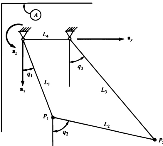
Figure P8.6

The system S formed by \boldsymbol{P}_{1} and P_{2} possesses only one degree of freedom in A. Hence, a single generalized coordinate, such as \pmb q_{1} , suffices to characterize the configuration of \boldsymbol{s} in \pmb{A} .However, it is convenient to introduce the pseudogeneralized' coordinates \pmb{q}_{2} and \pmb q_{3} (see Fig. P8.6), which must satisfy the configuration constraint equations

\begin{array}{r}{L_{1}\mathbf{c}_{1}+L_{2}\mathbf{c}_{2}-L_{3}\mathbf{c}_{3}=0}\\ {\qquad\qquad}\\ {L_{1}\mathbf{s}_{1}+L_{2}\mathbf{s}_{2}-L_{3}\mathbf{s}_{3}-L_{4}=0}\end{array}

and to let \pmb{u}_{2} and \pmb{u}_{3} be pseudo-generalized speeds defined as u_{2}\triangleq\dot{q}_{2} and u_{3}\triangleq\dot{q}_{3} Differentiationof theconstraintequationswithrespecttotimethenpermitsone to express \pmb{u}_{2} and \pmb{u}_{3} as in Eqs. (2.13.1), and \pmb{S} then canbetreated as if itwere a simple nonholonomic system.

Result

(\widetilde F_{1})_{\gamma}=\,-g L_{1}\biggl[m_{1}{\bf s}_{1}+m_{2}{\bf s}_{3}\,\frac{\sin(q_{2}\,-\,q_{1})}{\sin(q_{2}\,-\,q_{3})}\biggr]

8.7 Figure P8.7 shows 33 pin-connected rods, each of mass m andlength L suspended from a horizontal support. Contact forces of magnitudes Q,R_{:} and \boldsymbol{s} are applied to this system, as indicated in Fig. P8.7.

Using as generalized speeds the quantities L\dot{q}_{1},\;L\dot{q}_{2} , and L\dot{\boldsymbol{q}}_{3} , where \pmb q_{1} ， q2, and q3 are the angles shown in Fig. P8.7, determine the generalized active forces F_{1},F_{2} , and F_{3}

Results

\begin{array}{l}{F_{1}=(-Q+R+S)\mathbf{c}_{1}-30m g\mathbf{s}_{1}}\\ {F_{2}=(Q-R)\mathbf{c}_{2}-19m g\mathbf{s}_{2}}\\ {F_{3}=R\mathbf{c}_{3}-8m g\mathbf{s}_{3}}\end{array}

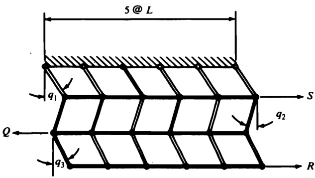
Figure P8.7

8.8 A rigid block B of length 2b and mass m is supported by two elastic beams, each of length L and flexural rigidity E I. The beams are “built in" both at thein supports and at the points P_{1} and P_{2} (Fig. P8.8).

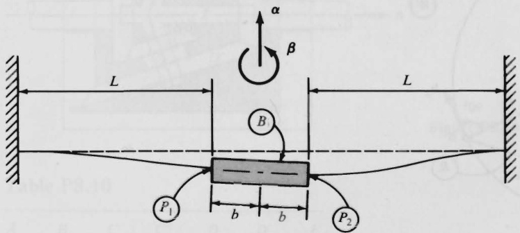
Figure P8.8

Confining attention to planar motions of B during which q_{1} and q_{2} ,the vertical beam displacements of \boldsymbol{P}_{1} and P_{2} ,respectively,remain small, one can treat B as a holonomic system possessing two degrees of freedom, and one can replace the set of contact forces exerted on B by the beam at the left with a couple of torque M_{1}\mathfrak{b} , together with a force V_{1}\alpha applied at \boldsymbol{P}_{1} ,where \pmb{\upalpha} and \upbeta are unit vectors directed as shown, and M_{1} and V_{1} are given by

\begin{array}{c}{{M_{1}=\displaystyle\frac{12E I}{L^{2}}\left(\displaystyle\frac{L}{3}\displaystyle\frac{q_{2}-q_{1}}{2b}-\displaystyle\frac{q_{1}}{2}\right)}}\\ {{V_{1}=\displaystyle\frac{12E I}{L^{3}}\left(q_{1}-\displaystyle\frac{L}{2}\displaystyle\frac{q_{2}-q_{1}}{2b}\right)}}\end{array}

The set of contact forces exerted on B by the beam at the right can be replaced similarly.

Taking for generalized speeds, u_{1} and u_{2} , the time-derivatives of q_{1} and q_{2} respectively, determine the generalized active forces F_{1} and F_{2}

Results

\begin{array}{l}{{F_{1}=\displaystyle\frac{12E I}{L^{3}}\left[-\left(1+\displaystyle\frac{L}{2b}+\displaystyle\frac{L^{2}}{6b^{2}}\right)\!q_{1}\right.\left.+\displaystyle\frac{L}{2b}\left(1+\displaystyle\frac{L}{3b}\right)\!q_{2}\right]+\displaystyle\frac{m g}{2}}}\\ {{F_{2}=\displaystyle\frac{12E I}{L^{3}}\left[\displaystyle\frac{L}{2b}\left(1+\displaystyle\frac{L}{3b}\right)\!q_{1}-\left(1+\displaystyle\frac{L}{2b}+\displaystyle\frac{L^{2}}{6b^{2}}\right)\!q_{2}\right]+\displaystyle\frac{m g}{2}}}\end{array}

8.9 The ends A and B of a uniform rod R of mass m are supported by a circular wire W that lies in a fixed vertical plane and has a radius r At thecenterofW,A and B subtend an angie 20 (Fig. P8.9).

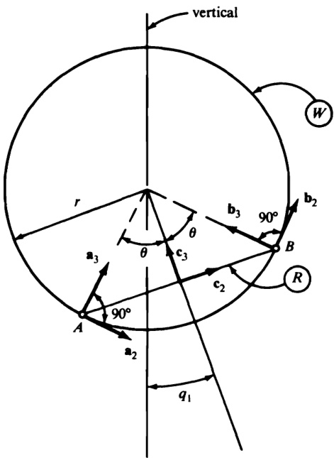
Figure P8.9

(a) Letting \pmb{u}_{1} be a generalized speed defined as u_{1}\triangleq\dot{q}_{1} ,where q_{1} is the angle shown in Fig. P8.9, and assuming that friction forces exerted on \pmb R by \pmb{W} at \pmb{A} and \pmb{B} are negligible, determine the generalized active force \boldsymbol{F}_{1}

(b) Letting -s T_{A}\mathbf{a}_{2} and -s T_{B}\mathbf{b}_{2} be friction forces exerted on \pmb R byW at \pmb{A} and \textbf{\emph{B}} , respectively, where T_{A} and T_{B} are non-negative quantities and s\triangleq {\pmb u}_{1}/|{\pmb u}_{1}| , while {\mathfrak{a}}_{2} and {\mathfrak{b}}_{2} are unit vectors directed as shown in Fig. P8.9, determine the generalized active force \boldsymbol{F}_{1}

(c) The forces exerted on \pmb R by \pmb{W} at \pmb{A} and \pmb{B} in the radial directions at these points can be expressed as N_{A}\mathbf{a}_{3} and N_{B}\mathbf{b}_{3} , respectively. To bring these into evidence in expressions for generalized active forces, let c be a reference frame in which the unit vectors \mathfrak{c}_{2} and \mathbf{c}_{3} shown in Fig. P8.9 are fixed, introduce generalized speeds u_{2} and \pmb{u}_{3} such that the velocity of the center of \pmb R in c is given by u_{2}\mathbf{c}_{2}+u_{3}\mathbf{c}_{3} , and determine the generalized active forces \boldsymbol{F}_{1},F_{2} , and \boldsymbol{F}_{3}

Results

\begin{array}{r l}&{F_{1}\,=\,-\,m g r\,\cos\,\theta\,\sin\,q_{1}}\\ &{F_{1}\,=\,-r[s(T_{A}\,+\,T_{B})\,+\,m g\,\cos\,\theta\,\sin\,q_{1}]}\\ &{F_{1}\,=\,-r[s(T_{A}\,+\,T_{B})\,+\,m g\,\cos\,\theta\,\sin\,q_{1}]}\\ &{F_{2}\,=\,-s(T_{A}\,+\,T_{B})\,\cos\,\theta\,+\,(N_{A}\,-\,N_{B})\,\sin\,\theta\,-\,m g\,\sin\,q_{1}}\\ &{F_{3}\,=\,s(T_{A}\,-\,T_{B})\,\sin\,\theta\,+\,(N_{A}\,+\,N_{B})\,\cos\,\theta\,-\,m g\,\cos\,q_{1}}\end{array}

8.10 Figure P.8.10 is a schematic representation of a reduction gear consisting of a fixed bevel gear \pmb{A} ,movingbevel gears B,C,C^{\prime},D,D^{\prime}, , and {\pmb E} , and an arm {\pmb F} ^{c} and \pmb{D} are rigidly connected to each other, as are C^{\prime} and \pmb{D^{\prime}} . The number of teeth of each gear is shown in Table P8.10.

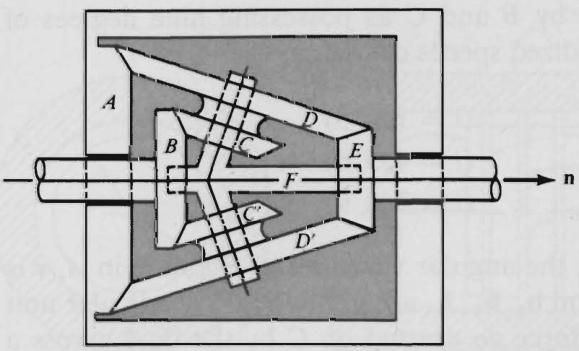
Figure P8.10

Table P8.10

<html>

A	B	C	C'	D	D'	E
60	30	30	30	61	61	20

</html>

Couples of torques T_{B}\mathbf{n} and T_{E}\mathbf{n} where n is a unit vector directed as shown in Fig. P8.10, are applied to the shafts carrying B and E , respectively. Letting u_{1} be a generalized speed defined as u_{1}\triangleq{\mathbf{\omega}}_{\mathbf{\omega}}^{A}\mathbf{\omega}^{B}\cdot\mathbf{n}. and assuming that rolling takes place at all points of contact between gears, determine the generalized active force F_{1}

8.11 A uniform sphere C of radius R is placed in a spherical cavity of a rigid body \mathcal{B} and B is free to move in a reference frame A as indicated in Fig. P8.11. The radius of the cavity exceeds R only slightly, and the space between B and C is filled with a viscous fluid.

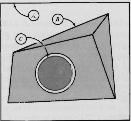
Figure P8.11

Regarding the system S formed by \pmb{B} and c as possessing nine degrees of freedom in A let u_{1},...,u_{9} be generalized speeds defined as

u_{i}\triangleq\left\{\!\!\begin{array}{l l}{{A_{\mathbf{0}}{}^{B}\cdot{\bf{b}}_{i}\quad}}&{{(i=1,2,3)}}\\ {{A_{\mathbf{0}}{}^{C}\cdot{\bf{b}}_{i-3}\quad}}&{{(i=4,5,6)}}\\ {{{\bf\!\!\!v}\cdot{\bf{b}}_{i-6}\quad}}&{{(i=7,8,9)}}\end{array}\!\!\right.

where \mathbf{\Delta}^{A}\mathbf{\omega}\mathbf{\mathsf{o}}^{B} and \mathbf{\deltaA_{GD}}c are, respectively, the angular velocities of \textbf{\emph{B}} and c in A,\,\mathbf{v} is the velocity of the center of c in \pmb{A} , and {\bf b}_{1},{\bf b}_{2},{\bf b}_{3} are mutually perpendicular unit vectors fixed in \pmb{B}. .Assume that the force do exerted on c by the fluid across a differential element \pmb{d}\pmb{\Sigma} of the surface c is given by

d\pmb{\upsigma}=\,-c^{B}\pmb{\upnu}^{P}\,d a

where c is a constant, \pmb{{\cal B}}_{\mathbf{v}}\pmb{{\cal P}} is the velocity in \pmb{B} of any point \pmb{P} of c lying within \pmb{d}\pmb{\Sigma} and da is the area of \pmb{d}\pmb{\Sigma} ; further, that at P the force exerted on \pmb{B} by the fuid across a differential element of the surface of the cavity is equal to \mathbf{\delta}-d\mathbf{\sigma}

Letting F_{1},...,F_{9} be the generalized active forces for s in \pmb{A} determine the contributions to F_{2} and \boldsymbol{F_{4}} of forces exerted on \pmb{B} and c by the fluid.

Results \scriptstyle{\frac{8}{3}}\pi c R^{4}(u_{5}\,-\,u_{2}) \scriptstyle{\frac{8}{3}}\pi c R^{4}(u_{1}\,-\,u_{4})

8.12 Referring to the example in Sec. 4.8, suppose that Q slides on P subject to the laws of Coulomb friction, and let \mu^{\prime} be the coefficient of kinetic friction for \pmb{A} and \pmb{P} . Under these circumstances, the quantities Q_{1},Q_{2} , and Q_{3} appearing in Eq. (4.8.14) can be expressed as functions of \mu^{\prime},R,M,g,e,f,\theta,u_{1},u_{2} , and a nonholonomic generalized active force {\widetilde{F}}_{3} associated with a generalized speed \pmb{u}_{3} introduced for the purpose of bringing Q_{1} into evidence. Taking u_{3}\triangleq\bar{r_{\omega^{A}}}\!\cdot\!\mathbf{a}_{3} , determine these functions.

Results

\begin{array}{r l}&{Q_{1}=(e M g\cos\theta-\tilde{F}_{3})/[f-\mu^{\prime}R u_{2}/({u_{2}}^{2}+f^{2}u_{1}\!^{2})^{1/2}]}\\ &{Q_{2}=-\mu^{\prime}u_{2}Q_{1}/({u_{2}}^{2}+f^{2}{u_{1}}^{2})^{1/2}}\\ &{Q_{3}=-\mu^{\prime}u_{1}f Q_{1}/({u_{2}}^{2}+f^{2}{u_{1}}^{2})^{1/2}}\end{array}

8.13 Figure P8.13 shows two views of a piston \pmb{P} of mass M in a cylinder c R_{1},R_{2} , and \pmb{R_{3}} are piston rings of thickness t, and \boldsymbol{t} is so small in comparison with \pmb R , the internal radius of c , that the contacts between \boldsymbol{R}_{1},\,\boldsymbol{R}_{2},\,\boldsymbol{R}_{3} and c can be regarded as taking place along circles of radius \pmb R . The axis of ^{c} is horizontal and parallel to a unit vector i, and P is subjected to the action of a set of contact forces equivalent to a force E\mathbf{i} applied to P at P^{*} , the mass center of \pmb{P}

Two generalized speeds, \pmb{u}_{1} and \pmb{u}_{2} , defined as

u_{1}\triangleq\mathbf{\omega}\bullet\mathbf{i}\qquad u_{2}\triangleq\mathbf{v}^{\ast}\cdot\mathbf{i}

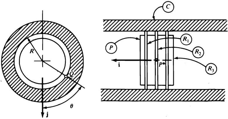
Figure P8.13

where の is the angular velocity of \pmb{P} in c and \mathbf{v}^{*} is thevelocity of \scriptstyle P^{*} in c characterizemotions of \pmb{P} in C if P is free to rotate and translate. A third generalized speed, \pmb{u}_{3} , defined as

u_{3}\triangleq\mathbf{v}^{\ast}\cdot\mathbf{j}

where j is a unit vector directed vertically downward, can be introduced to bring into evidence radial contact forces exerted on R_{1},R_{2} ,and R_{3} by C

Assumingthat \pmb{n} , the contact pressure (force per unit of length) at a point Q situated on any one of R_{1},R_{2} ,or R_{3} as shown in Fig. P8.13, is given by

n=\alpha+\beta\cos\!\left(\!\frac{\theta}{2}\!\right)\!\qquad(-\pi\leq\theta\leq\pi)

where \pmb{\alpha} and \beta are constants, and letting \pmb{\mu}^{\prime} be the coefficient of kinetic friction for c and \boldsymbol{R}_{1},\,\boldsymbol{R}_{2},\,\boldsymbol{R}_{3} , determine the generalized active forces F_{1},\,F_{2} , and F_{3} for motions during which {\pmb u}_{3}={\bf0}

Results

\begin{array}{l c l}{F_{1}=-6\mu^{}R^{3}(\pi\alpha+2\beta)u_{1}[(R u_{1})^{2}+{u_{2}}^{2}]^{-1/2}}\\ {F_{2}=-6\mu^{}R(\pi\alpha+2\beta)u_{2}[(R u_{1})^{2}+{u_{2}}^{2}]^{-1/2}+E}\\ {F_{3}=-4R\beta+M g}\end{array}

\mathbf{*8.14} Referring to Problem 3.15 (see also Problem 4.17), let A^{*},\,B^{*},\,C^{*},\,D^{*} be the mass centers of A,B,C,D , respectively, and designate as m_{A} ， m_{B} ， m_{c} ， m_{D} the masses of A, B, C, D, respectively. The pinion gears have negligible masses. To drive the robot arm, forces are transmitted from E to \pmb{A} via a motor (not shown in Fig. P3.15). The set of all such forces is equivalent to a couple of torque TE/A together with a force KE/A applied to A at a point on the axis of the hub. The set of forces exerted by \pmb{A} on \pmb{B} by means of the motor connecting \pmb{A} to \pmb{B} at P is equivalent to a couple of torque \mathbf{T}^{A/B} together with a force \mathbf{K}^{A/B} applied to \pmb{B} at \pmb{P}. Finally, the set of forces exerted by \pmb{B} on c through the rack-and-pinion drive is equivalent to a couple of torque TB/C together with a force KB/C applied to C at C*.

306 PROBLEM SETS

Expressing \cdot\,\mathbf{T}^{E/A},\,\mathbf{K}^{E/A},\,\mathbf{T}^{A/B},\,\mathbf{K}^{A/B},\,\mathbf{T}^{B/C} , and \mathbf{K}^{B/C} as, respectively,

\begin{array}{r l}&{\mathbf{T}^{E/A}=T_{1}^{\phantom{A}E/A}\mathbf{a}_{1}+T_{2}^{\phantom{A}E/A}\mathbf{a}_{2}+T_{3}^{\phantom{E}\!\!E/A}\mathbf{a}_{3}}\\ &{\mathbf{K}^{E/A}=K_{1}^{\phantom{A}E/A}\mathbf{a}_{1}+K_{2}^{\phantom{E}\!\!E/A}\mathbf{a}_{2}+K_{3}^{\phantom{A}E/A}\mathbf{a}_{3}}\\ &{\mathbf{T}^{A/B}=T_{1}^{\phantom{A}/B}\mathbf{b}_{1}+T_{2}^{\phantom{A}/B}\mathbf{b}_{2}+T_{3}^{\phantom{A}/B}\mathbf{b}_{3}\,.}\\ &{\mathbf{K}^{A/B}=K_{1}^{\phantom{A}/B}\mathbf{b}_{1}+K_{2}^{\phantom{A}/B}\mathbf{b}_{2}+K_{3}^{\phantom{A}/B}\mathbf{b}_{3}}\\ &{\mathbf{T}^{B/C}=T_{1}^{\phantom{B}/C}\mathbf{b}_{1}+T_{2}^{B/C}\mathbf{b}_{2}+T_{3}^{\phantom{B}/C}\mathbf{b}_{3}}\\ &{\mathbf{K}^{B/C}=K_{1}^{\phantom{B}/C}\mathbf{b}_{1}+K_{2}^{\phantom{B}/C}\mathbf{b}_{2}+K_{3}^{\phantom{B}/C}\mathbf{b}_{3}}\end{array}

and letting \pmb{g} be the local gravitational acceleration, determine the generalized active forces \boldsymbol{F}_{1},\boldsymbol{F}_{2} , and F_{3} for the robot arm in \pmb{E} ,where \boldsymbol{F}_{i} is associated with the generalized speed u_{i}\,(i=1,2,3) defined in Problem 3.15.

Results

\begin{array}{l}{{F_{1}=T_{1}^{~E/A}}}\\ {{{\cal F}_{2}=T_{2}^{~A/B}-g[(m_{B}L_{B}+m_{C}Z_{9}+m_{D}Z_{14}){\bf c}_{1}-m_{D}p_{1}{\bf s}_{1}]}}\\ {{{\cal F}_{3}=K_{3}^{~B/C}-g(m_{C}+m_{D}){\bf s}_{1}}}\end{array}

8.15 Letting S be the set of two particles \boldsymbol{P}_{1} and P_{2} considered in Problem 8.1, form expressions for the generalized inertia forces F_{1}{}^{*},F_{2}{}^{*}; {{F}_{3}}^{*} for \pmb{s} in \pmb{A}_{:} doing so for each of the three sets of generalized speeds defined in Problem 8.1. Comment briefly on the relative merits of the three sets of generalized speeds.

Results

F1* = {-(m + m2)(u sec wt + 2wq1 tan wt) \mathbf{\nabla}+\,m_{2}[(\omega^{2}+{u_{3}}^{2}){\mathbf{c}}_{3}\,+\,\dot{u}_{3}\,{\mathbf{s}}_{3}]\} secwot \begin{array}{r l}&{\ {F_{2}}^{*}=-(m_{1}+m_{2})\hat{u}_{2}+L m_{2}(u_{3}^{2}s_{3}-\hat{u}_{3}{\bf c}_{3}),}\\ &{\ {F_{3}}^{*}=-m_{2}L[L(\hat{u}_{3}+\omega^{2}s_{3}{\bf c}_{3})-(\hat{u}_{1}\ \mathrm{sgc}\ \omega t+2\omega\hat{q}_{1}\ \mathrm{tan}\ \omega t)s_{3}+}\\ &{\ {F_{1}}^{*}=-(m_{1}+m_{2})(\hat{u}_{1}-\omega^{2}q_{1}c_{3}-u_{2}u_{3})+L m_{2}(\omega^{2}c_{3}^{2}+u_{3}^{2})}\\ &{\ {F_{2}}^{*}=-(m_{1}+m_{2})(\hat{u}_{2}+u_{3}u_{1}+\omega^{2}q_{1}s_{3})-L m_{2}(\hat{u}_{3}+\omega^{2}s_{3}c_{3})}\\ &{\ {F_{3}}^{*}=-m_{2}L[\hat{u}_{2}+u_{3}u_{1}+\omega^{2}q_{1}s_{3}+L(\hat{u}_{3}+\omega^{2}s_{3}c_{3})]\ \ \ }\\ &{\ {F_{1}}^{*}=-(m_{1}+m_{2})(\hat{u}_{1}-\omega^{2}q_{1})+L m_{2}(\omega^{2}c_{3}+\hat{u}_{3}s_{3}+u_{3}^{2}c_{3})}\\ &{\ {F_{2}}^{*}=-(m_{1}+m_{2})\hat{u}_{2}+L m_{2}(u_{3}^{2}s_{3}-\hat{u}_{3}c_{3})}\\ &{\ {F_{3}}^{*}=-m_{2}L[(\hat{u}_{3}^{*}+\omega^{2}s_{3}c_{3})-(\hat{u}_{1}-\omega^{2}q_{1})s_{3}+\hat{u}_{2}c_{3}]}\end{array} u2c3]

8.16 Making the same assumptions as in Problem 8.2, use Eqs. (4.11.1) to determine the generalized inertia forces \widetilde{\pmb F}_{1}{}^{*} and \widetilde{F}_{2}{}^{*} forS in \pmb{A} Check the results by using Eqs. (4.11.4) in conjunction with results from Problem 8.15, and comment briefly on the relative merits of Eqs. (4.11.1) and Eqs. (4.11.4).

Results

\begin{array}{r l}&{\widetilde{F}_{1}^{\;\ast}=(m_{1}+m_{2})(\omega^{2}q_{1}\mathrm{c}_{3}-\dot{u}_{1})-m_{1}{u_{2}}^{2}/L+m_{2}L\omega^{2}\mathrm{c}_{3}^{2}}\\ &{\widetilde{F}_{2}^{\;\ast}=\,-m_{1}(\dot{u}_{2}+\omega^{2}q_{1}\mathrm{s}_{3}-u_{1}u_{2}/L)}\end{array}

8.17. The system S considered in the example in Sec. 4.8 and shown in Fig. 4.8.1 has the following inertia properties: \pmb{A} has a mass m_{A} and moment of inertia \boldsymbol{I_{A}} about a line parallel to {\bf a}_{1} and passing through the mass center A^{*} of \pmb{A} , which is situated on line \pmb{D}\pmb{E} at a distance \pmb{a} from point \pmb{D} .The wheels \pmb{B} and c each have a mass m_{B} and moment of inertia J about the line joining the wheel centers (which are the wheels' mass centers and are separated by a distance 2b ), and each wheel has a moment of inertia \pmb{K} about any line that passes through the center of the wheel and is perpendicular to the line joining the wheel centers.

Defining generalized speeds \pmb{u}_{1} and \pmb{u}_{2} as in Eqs. (4.8.9), and \pmb{u}_{3} as in Problem 8.12, determine the generalized inertia forces \widetilde{\boldsymbol{F}}_{1}{}^{*},\widetilde{\boldsymbol{F}}_{2}{}^{*} and {\tilde{F}}_{3}{}^{*} for s in {\pmb F}

Results

\begin{array}{l}{{\tilde{F}_{1}{}^{*}=\,-(I_{A}+2J b^{2}/R^{2}+2K+m_{A}a^{2}+2m_{B}b^{2})\dot{u}_{1}\,-\,m_{A}a u_{1}u_{2}}}\\ {{{\tilde{F}}_{2}{}^{*}=\,-(m_{A}+2m_{B}+2J/R^{2})\dot{u}_{2}\,+\,m_{A}{a u_{1}}^{2}}}\\ {{{\tilde{F}}_{3}{}^{*}=0}}\end{array}

\mathbf{*8.18} The equations that follow furnish useful expressions for \mathbf{T}^{*} , the inertia torque for a rigid body \pmb{B} in a reference frame \pmb{A}. Establish the validity of each of these equations.

^{(a)} When \mathbf{\delta}^{\mathbf{o}} the angular velocity of \pmb{B} in \pmb{A} , can be expressed as {\bf{\omega}}{\bf{\omega}}{\bf{\omega}}{\bf{\omega}}{\bf{\omega}} ， where \mathbb{n}_{a} is a unit vector fixed in \pmb{A} , then

{\bf T}^{*}=\,-\dot{\omega}I_{a}{\bf n}_{a}+(\omega^{2}I_{c a}-\dot{\omega}I_{a b}){\bf n}_{b}-(\omega^{2}I_{a b}+\dot{\omega}I_{c a}){\bf n}_{c}\,\,.

where \mathbb{n}_{b} and \mathfrak{n}_{c} are unit vectors perpendicular to \mathbb{n}_{a} and to each other, and are oriented such that \begin{array}{r}{\bar{\mathbf{n}}_{a}=\mathbf{n}_{b}\,\times\,\mathbf{n}_{c};\,I_{a}}\end{array} is the central moment of inertia of \pmb{B} with respect to a line parallel to \begin{array}{r}{\mathbf{n}_{a};I_{a b}}\end{array} is the central product of inertia of \pmb{B} for \mathbb{n}_{a} and \mathbb{n}_{b} ; and I_{c a} is the central product of inertia of \textbf{\emph{B}} for \mathbf{n}_{c} and \mathbb{n}_{a}

(b) If {\bf b}_{1} {\bf b}_{2} {\bf b}_{3} form a right-handed set of mutually perpendicular unit vectors fixed in \pmb{B} and \omega_{i}\triangleq\omega\cdot\mathbf{b}_{i}\,(i=1,2,3) ,where \pmb{\omega} is the angular velocity of \pmb{B} in \pmb{A} then

\begin{array}{r l}&{\mathbf{T}^{*}=\mathbf{\Phi}-[I_{11}\dot{\omega}_{1}+I_{12}\dot{\omega}_{2}+I_{13}\dot{\omega}_{3}+(I_{31}\omega_{2}-I_{12}\omega_{3})\omega_{1}}\\ &{\phantom{...}+I_{23}({\omega_{2}}^{2}-{\omega_{3}}^{2})+(I_{33}-I_{22})\omega_{2}\omega_{3}]\mathbf{b}_{1}}\\ &{\phantom{...}-[I_{22}\dot{\omega}_{2}+I_{23}\dot{\omega}_{3}+I_{21}\dot{\omega}_{1}+(I_{12}\omega_{3}-I_{23}\omega_{1})\omega_{2}}\\ &{\phantom{...}+I_{31}({\omega_{3}}^{2}-{\omega_{1}}^{2})+(I_{11}-I_{33})\omega_{1}]\mathbf{b}_{2}}\\ &{\phantom{...}-[I_{33}\dot{\omega}_{3}+I_{31}\dot{\omega}_{1}+I_{32}\dot{\omega}_{2}+(I_{23}\omega_{1}-I_{31}\omega_{2})\omega_{3}}\\ &{\phantom{...}+I_{12}({\omega_{1}}^{2}-{\omega_{2}}^{2})+(I_{22}-I_{11})\omega_{1}\omega_{2}]\mathbf{b}_{3}\quad\quad\cdot}\end{array}

where I_{j k} is the central inertia scalar for \ensuremath{\mathbf{b}}_{j} and {\mathfrak{b}}_{k}\,(j,k=1,2,3)

(c) If \mathbf{H} is the central angular momentum of \textbf{\emph{B}} in \pmb{A} ,then

\mathbf{T}^{*}=\mathbf{-\,}^{A}\mathbf{\caldH}

{}^{*}\!8.19\ (\widetilde{F}_{r}{}^{*})_{B} , the contribution of a rigid body \pmb{B} to the generalized inertia force \widetilde{F}_{r}{^{*}}\left(r=1,\ldots,p\right) in a reference frame \pmb{A} , can be expressed as

(\widetilde{F}_{r}{^*})_{B}=\tilde{\upomega}_{r}\cdot\mathrm{T}^{Q}+\tilde{\upnu}_{r}{^0}\cdot\mathbf{R}{^*}\qquad(r=1,\ldots,p)

where \tilde{\pmb{\upsigma}}_{r} and \mathbf{R}^{\ast} are defined as in connection with Eqs. (4.11.7), but \mathbf{T}^{Q} and \tilde{\mathbf{v}}_{r}^{\,Q} differ from \mathbf{T}^{*} and \tilde{\mathbf{v}}_{r}^{\ast} , respectively, being defined as follows : Let Q be a point of \pmb{B} \mathbf{r}^{Q P_{i}} the position vector from Q to a generic particle \boldsymbol{P}_{i} of \mathbfit{B} m_{i} the mass of \boldsymbol{P_{i}} ， and {\bf{a}}_{i} the acceleration of P_{i}\,(i=1,\ldots,\beta) in reference frame \pmb{A} . Then

\mathbf{T}^{Q}\triangleq\mathrm{~-~}\sum_{i\,=\,1}^{\beta}m_{i}\mathbf{r}^{Q P_{i}}\,\times\,\mathbf{a}_{i}

while \tilde{\mathbf{v}}_{r}^{\textit{Q}} is the rth nonholonomic partial velocity of Q in \pmb{A} . Furthermore, \mathbf{T}^{Q} [compare with \mathbf{T}^{*} as given in Eq. (4.11.8)] can be expressed as

{\bf T}^{Q}=\mathrm{}-m{\bf r}^{Q B^{*}}\times{\bf\nabla}{\bf a}^{Q}-\alpha\cdot{\bf I}^{Q}-\mathrm{\bf~\infty~}\times{\bf\nabla}{\bf I}^{Q}\cdot\mathrm{\bf\odot}

where m is the mass of B,{\bf r}^{Q B^{*}} is the position vector from Q to B^{*},\mathbf{a}^{Q} is the acceleration of Q in A,\pmb{\alpha} and \mathbf{\delta}^{\mathbf{o}} are, respectively, the angular acceleration of \pmb{B} in \pmb{A} and the angular velocity of \boldsymbol{B} in \pmb{A} and \mathbf{\Delta}\mathbf{R} is the inertia dyadic of \textbf{\emph{B}} relative to Q

Establish the validity of Eqs. (a) and (c), and devise an example to illustrate the utility of these relationships.

\mathbf{*8.20} Referring to Problem 3.15 (see also Problems 4.17 and 8.14), let A,\,B,\,C, and \pmb{D} have the following mass distribution properties. The central principal axes of \pmb{A} are parallel to {\bf a}_{1},{\bf a}_{2},{\bf a}_{3} (see Fig. P3.15), and the associated moments of inertia have the values A_{1},\,A_{2} \boldsymbol{A}_{3} , respectively. The central principal axes of \pmb{B} and c are parallel to \ensuremath{\mathbf{b}}_{1},\,\ensuremath{\mathbf{b}}_{2} {\bf b}_{3} (see Fig. P3.15), and the associated moments of inertia have the values B_{1},\,B_{2}, B_{3} and C_{1},\,C_{2},\,C_{3} , respectively. Central inertia scalars D_{i j}\left(i,j=1,2,3\right) for \pmb{D} are defined as

D_{i j}\triangleq\mathbf{b}_{i}\cdot\mathbf{I}^{D}\cdot\mathbf{b}_{j}\qquad(i,j=1,2,3)

where \mathbf{I}^{D} is the central inertia dyadic of \pmb{D}

Letting \mathbf{T}_{A}{}^{*},\,\mathbf{T}_{B}{}^{*},\,\mathbf{T}_{C}{}^{*} , and \mathbf{T}_{\pmb{p}}* denote the inertia torques for A,B,C_{:} and \pmb{D} in E , express {{\mathbf{T}}_{{\pmb{A}}}}^{*} in terms of {\bf a}_{1},{\bf a}_{2},{\bf a}_{3} , and \mathbf{T}_{B}^{\ast},\mathbf{T}_{C}^{\ast},\mathbf{T}_{D}^{\ast} in terms of \mathbf{b}_{1},\mathbf{b}_{2},\mathbf{b}_{3}

To facilitate the writing of results, introduce k_{1},\ldots,k_{16} and Z_{35},\ldots,Z_{54} as

\begin{array}{r l}{k_{1}\triangleq B_{2}-B_{3},\quad k_{2}\triangleq B_{3}-B_{1}\quad k_{3}\triangleq B_{1}-B_{2}\quad k_{4}\triangleq C_{2}-C_{3}}\\ {k_{3}\triangleq C_{3}-C_{1},\quad k_{4}\triangleq C_{1}-C_{2}\quad k_{7}\triangleq D_{3}-D_{2},\quad k_{8}\triangleq B_{1}-D_{3}}&{k_{9}\Delta_{11}-D_{3}}\\ {k_{9}\triangleq B_{22}-D_{11}\quad k_{10}\triangleq B_{11}+k_{11}\quad k_{11}\triangleq B_{3}-k_{3},\quad k_{12}\triangleq C_{1}+k_{4},}\\ {k_{13}\triangleq C_{3}-k_{6}\quad k_{14}\triangleq D_{11}-k_{7}\quad k_{15}\triangleq D_{31}+D_{13}\quad k_{16}\triangleq D_{33}\,,}\\ {\quad L_{3}\triangleq\hat{x}_{1,B_{1}}\quad Z_{36}\triangleq Z_{3,k_{10}}\quad Z_{37}\triangleq Z_{2}\quad Z_{3}\quad\hat{z}_{3}\triangleq-Z_{37}\hat{k}_{2}}\\ {Z_{3}\triangleq_{3}B_{3},\quad Z_{40}\triangleq Z_{4}k_{11}\quad Z_{41}\triangleq\hat{c}_{1}\tau_{1}\quad Z_{42}\triangleq Z_{3}k_{12}\quad\quad Z_{43}\ne Z_{3}k_{12}\quad\quad}\\ {Z_{43}\triangleq-Z_{37},\quad k_{5}\quad Z_{44}\triangleq\hat{s}_{1,C_{3}}\quad Z_{43}\triangleq Z_{4}k_{13}\quad Z_{46}\triangleq Z_{4}\quad\hat{z}_{1}^{2}}\\ {Z_{47}\triangleq u_{2}^{2}\quad Z_{48}\triangleq\hat{z}_{2}\quad Z_{49}\triangleq\hat{D}_{11}\varsigma_{1}+D_{13}\}}\\ {Z_{50}\triangleq\hat{k}_{14}Z_{3}+k_{15}Z_{4}-D_{12}\hat{z}_{37}+D_{23}(Z_{47}-Z_{48})\quad Z_{31}\triangleq D_{23}\hat{\mathbf{z}}_{1}

Results

\begin{array}{r l}&{\mathbf{T}_{A}^{\ast}=-\dot{u}_{1}A_{1}\mathbf{a}_{1}}\\ &{\mathbf{T}_{B}^{\ast}=\mathbf{\Phi}-(\dot{u}_{1}Z_{35}+Z_{36})\mathbf{b}_{1}-(\dot{u}_{2}B_{2}+Z_{38})\mathbf{b}_{2}-(\dot{u}_{1}Z_{39}+Z_{40})\mathbf{b}_{3}}\\ &{\mathbf{T}_{C}^{\ast}=\mathbf{\Phi}-(\dot{u}_{1}Z_{41}+Z_{42})\mathbf{b}_{1}-(\dot{u}_{2}C_{2}+Z_{43})\mathbf{b}_{2}-(\dot{u}_{1}Z_{44}+Z_{45})\mathbf{b}_{3}}\\ &{\mathbf{T}_{D}^{\ast}=\mathbf{\Phi}-(\dot{u}_{1}Z_{49}+\dot{u}_{2}D_{12}+Z_{50})\mathbf{b}_{1}-(\dot{u}_{1}Z_{51}+\dot{u}_{2}D_{22}+Z_{52})\mathbf{b}_{2}}\\ &{\quad\quad-\mathbf{\Phi}(\dot{u}_{1}Z_{53}+\dot{u}_{2}D_{32}+Z_{54})\mathbf{b}_{3}}\end{array}

\mathbf{*8.21} Referring to Problem 3.15 (see also Problem 4.17, 8.14, and 8.20), determine the generalized inertia forces F_{1}{}^{*},\,F_{2}{}^{*} ,and {{F}_{3}}^{*} for the robot arm in E_{\mathrm{{*}}} where \boldsymbol{F}_{i}^{\ast} is associated with the generalized speed u_{i}\,(i=1,2,3)

Results

\begin{array}{r l}{F_{1}^{*}=-\dot{u}_{1}[A_{1}+\mathrm{c}_{1}(Z_{3}*+Z_{41}+Z_{49})+s_{1}(Z_{39}+Z_{44}+Z_{53})}\\ {+}&{}\\ {-\dot{u}_{1}Z_{4}^{L}+m_{B}Z_{6}^{2}+m_{C}Z_{10}^{*}{}^{2}+m_{D}(Z_{13}^{*}{}^{2}+Z_{15}^{2}+Z_{16}^{2})]}\\ {-\dot{u}_{2}[\mathrm{c}_{1}D_{12}+s_{1}D_{32}+m_{D}(Z_{13}\mathrm{Z}_{14}-Z_{16}p_{1})]-\dot{u}_{3}m_{D}Z_{16}}\\ {-[\mathrm{c}_{1}(Z_{36}+Z_{42}+Z_{50})+s_{1}(Z_{40}+Z_{45}+Z_{54})+m_{B}Z_{6}Z_{23}}\\ {+}&{}\\ {+}&{}\\ {\dot{\tau}_{2}^{*}=-\dot{u}_{1}[Z_{51}+m_{D}(Z_{13}\mathrm{Z}_{32}+Z_{15}\mathrm{Z}_{33}+Z_{16}Z_{34})]}\\ {+}&{}\\ {+}&{}\\ {+m_{C}Z_{9}^{2}+m_{D}(Z_{14}^{*}{}^{2}+p_{1}^{2})]+\dot{u}_{3}m_{D}p_{1}-[Z_{38}+Z_{22}+m_{B}L_{8}^{2}}\\ {+}&{}\\ {+m_{B}L_{B}Z_{22}+m_{C}Z_{9}Z_{26}+m_{D}(Z_{14}Z_{32}-p_{1}Z_{34})]}\\ {\tilde{\mathrm{c}}_{3}^{*}=-\dot{u}_{1}m_{D}Z_{16}+\dot{u}_{2}m_{D}p_{1}-\dot{u}_{3}(m_{C}+m_{D})-(m_{C}Z_{38}+m_{D}Z_{34})}\end{array}

\mathbf{*8.22} Letting \boldsymbol{s} be a simple nonholonomic system possessing generalized coordinates q_{1},\ldots,q_{n} and generalized speeds u_{1},\dotsc,u_{p} in a reference frame \pmb{A} ， and letting G be the Gibbs function for s in \pmb{A} (see Problem 6.16), show that the generalized inertia forces \widetilde{F}_{1}{}^{*},...,\widetilde{F}_{p}{}^{*} for s .n \pmb{A} can be expressed as

\widetilde{F}_{r}{}^{*}=\,-\,\frac{\partial G}{\partial\dot{u}_{r}}\qquad(r=1,\ldots,p)

近 G is regarded as a function of q_{1},\ldots,q_{n},u_{1},\ldots,u_{p}, and \dot{u}_{1},...,\dot{u}_{p} [The formula developed in Problem 6.16 can be used in conjunction with the present result to find the contribution of a rigid body \pmb{B} to. \tilde{F_{r}}^{*}\;(r=1,\ldots,p) . When using the formula for this purpose, one can omit the term \omega^{2}\boldsymbol{\omega}\cdot\mathbf{I}\cdot\mathbf{\omega} for this term does not contain any of \dot{u}_{1},...,\dot{u}_{p} , and hence cannot contribute to \partial G/\partial{\dot{u}}_{r}\,(r=1,\dots,p).]

PROBLEM SET 9

(Secs. 5.1-5.3)

9.1 A system S of two particles \boldsymbol{P}_{1} and \scriptstyle P_{2} of masses m_{1} and m_{2} moves in such a way that the distance r between P_{1} and P_{2} is free to vary with time. Assuming that no forces act on P_{1} and P_{2} other than the gravitational forces exerted by the particles on each other, show that -G m_{1}m_{2}/r+C_{!} where G is the universal gravitational constant and c is any function of time, is a potential energy of S.

9.2 A uniform thin rod \pmb R of cross-sectional area \pmb{A} is partially immersed in a fluid of mass density \rho.R can move in such a way that \pmb q_{1} , the distance from the immersed end of \pmb R to the surface of the fluid, and q_{2} , the angle between the axis of \pmb R and the local vertical, are free to vary. Letting \beta be the set of buoyancy forces exerted on \pmb R by the fuid, show that g\rho A(q_{1}{}^{2}/2) sec \pmb q_{2} is a potential energy contribution of \beta for \pmb R

\bf{*9.3} Referring to Problem 2.7, suppose that C is of uniform density and has a mass ^{m} and let be the set of gravitational forces acting on c Verify that mgR cos q_{2} is a potential energy contribution of \gamma for c and show that this function is a potential energy of ^{c} in \pmb{A} when ^{c} is rolling on \pmb{H} , but not when slipping is taking place at \pmb{P} , unless the contact between \pmb{H} and \pmb{P} is frictionless. (Expressions for generalized active forces are available in Problem 8.3.)

9.4 Show that -g(m_{1}L_{1}\mathsf{c}_{1}+m_{2}L_{3}\mathsf{c}_{3}) is a potential energy of the system of two particles considered in Problem 8.6. Verify that the expression for (\widetilde{F}_{1})_{\gamma} found in Problem 8.6 can be obtained by replacing {\widetilde{\pmb F}}, with \(\widetilde{F}_{r})_{v} , and \pmb{V} with -g(m_{1}L_{1}{\mathsf{c}}_{1}+m_{2}L_{3}{\mathsf{c}}_{3}), in Eqs. (5.1.14).

9.5 Referring to Problem 8.7, determine with the aid of Eq. (5.2.2) a potential energy contribution V_{\gamma} of the gravitational forces acting on the 33 bars; use Eqs. (5.1.2) with V replaced with V_{\gamma} and F_{r} replaced with (F_{r})_{\gamma} to find the contributions (F_{r})_{\gamma} of the gravitational forces to the generalized active forces F_{r} (r=1,2,3) Comment briefly on the relative merits of the method used to obtain these contributions in Problem 8.7, on the one hand, and the method employed in the present problem, on the other hand.

9.6 Construct a potential energy V of the system described in Problem 8.8.

Result

V=\frac{6E I}{L^{3}}\left[\left(1+\frac{L}{2b}+\frac{L^{2}}{6b^{2}}\right)({q_{1}}^{2}+{q_{2}}^{2})-\frac{L}{b}\left(1+\frac{L}{3b}\right)q_{1}q_{2}\right]-\frac{m g}{2}\,(q_{1}+q_{2})

9.7 Referring to Problem 8.9, suppose that the plane containing W is made to rotate with a prescribed angular speed about a vertical line passing through the center of W. Showthat-mgr cos \boldsymbol{\theta} cOS q_{1} is a potential energy of R solongasthe contactsbetween R and W at A and B areperfectlysmooth.

\mathbf{*9.8} Referring to the example in Sec. 4.8 (seeFig.4.8.1), let q_{1} be the angle between \mathbf{n}_{2} and {\mathbf a}_{2} (see Fig. 4.8.2) as before; define q_{2} and q_{3} as

q_{2}\triangleq\mathbf{p}\cdot\mathbf{n}_{2}\qquad q_{3}\triangleq\mathbf{p}\cdot\mathbf{n}_{3}

where \mathbf{p} is the position vector from a point fixed in F to point D ;and introduce wheelrotation angles q_{4} and q_{5} as shown in Fig. P9.8, where L_{B} and L_{c} arelines fixed in B and C , respectively. Assume that no friction forces come into play at

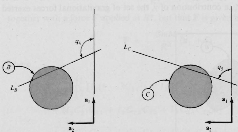
Figure P9.8

point Q in Fig. 4.8.1, and that B and C are driven by motors attached to A in such a way that the sets of contact forces exerted by A on B andby A on C are equivalent to couples of torques {\bf{T}}_{B} and {{\bf{T}}_{C}} ,respectively,with

{\bf T}_{B}=\,T_{B}{\bf a}_{3}\qquad{\bf T}_{C}=\,T_{C}{\bf a}_{3}

where T_{B} and T_{C} are functions of q_{1},\ldots,q_{5}

Show that V(q_{\lambda},\dots,q_{s},t) is a potential energy of s in F if

{\frac{\partial V}{\partial q_{1}}}+{\frac{b}{R}}\left({\frac{\partial V}{\partial q_{4}}}-{\frac{\partial V}{\partial q_{5}}}\right)={\frac{b}{R}}\left(T_{\mathrm{C}}-T_{B}\right)-\,M g e\sin\,\theta\mathbf{c}_{1}

\frac{\partial V}{\partial q_{2}}\,{\bf c}_{1}+\frac{\partial V}{\partial q_{3}}\,{\bf s}_{1}+\frac{1}{R}\left(\frac{\partial V}{\partial q_{4}}+\frac{\partial V}{\partial q_{5}}\right)={}-\frac{1}{R}\,(T_{\mathrm{c}}+T_{B})-M g\,\sin\,\theta{\bf s}_{1}

9.9 In Fig. P9.9, P is a particle fixed in a reference frame A ,and B^{*} is the mass center of a rigid body B;\mathbf{a}_{1},\mathbf{a}_{2}, {\mathbf{a}}_{3} form a right-handed set of mutually perpendicular unit vectors such that {\bf a}_{1} points from P to B^{*};\,\mathbf{b}_{1},\,\mathbf{b}_{2},\,\mathbf{b}_{3} form a similar set of unit vectors parallel to central principal axes of B

Assume throughout what follows that the set \gamma of all gravitational forces exertedby P on B can be replaced with a couple of torque \mathbf{T} givenby

\mathbf{T}=\frac{3G m}{R^{3}}\,\mathbf{a}_{1}\,\times\,\mathbf{I}\cdot\mathbf{a}_{1}

together with a force \mathbf{F} applied at B^{*} and given by

\mathbf{F}=\mathbf{-}\,{\frac{G m M}{R^{2}}}\,\mathbf{a}_{1}

where G is the universal gravitational constant, m is the mass of P,R is the distance from P to B^{*} Iis the central inertia dyadic of B and M is themass of B

(a) If {\bf a}_{1} {\mathbf a}_{2} , and {\bf a}_{3} are fixed in A and the orientation of B in A is specified in terms of three angles q_{1},q_{2},q_{3} like those used in Problem 1.1 to orient D in A (see Fig. P1.1), then V_{\gamma} ,a contribution of \gamma the setofgravitational forcesexerted

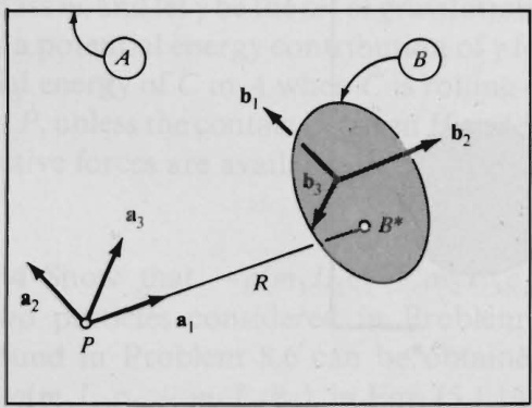
Figure P9.9

by \pmb{P} on \pmb{B} toapotential energyof \textbf{\emph{B}} in \pmb{A} can be expressed in terms of q_{1},q_{2},q_{3} solongas B^{*} iskept fixed in \pmb{A} Defininggeneralizedspeeds u_{1},u_{2},u_{3} for \pmb{B} in \pmb{A} as

u_{i}\triangleq A_{\pmb{\omega}}^{\b\Delta}\pmb{\omega}^{B}\cdot\mathbf{b}_{i}\qquad(i=1,2,3)

and letting I_{j}\triangleq\mathbf{b}_{j}\cdot\mathbf{I}\cdot\mathbf{b}_{j}\ \left(j=1,2,3\right) determine V_{\gamma}

(b) Use the result of part (a) to determine (F_{1})_{\gamma},(F_{2})_{\gamma},(F_{3})_{\gamma} , the contributions of \gamma to the generalized active forces for \pmb{B} in \pmb{A} corresponding to generalized speeds u_{1},u_{2},u_{3} defined as

u_{i}\triangleq\dot{q}_{i}\qquad(i=1,2,3)

(c) Assuming that {\bf a}_{1},{\bf a}_{2} , and {\bf a}_{3} are fixed in \pmb{A} , but that B^{*} can move in \pmb{A} along line \pmb{P}\pmb{B}^{\ast} , which means that \pmb{B} has four degrees of freedom in \pmb{A} , show that V_{\gamma} does not exist.

Results

\begin{array}{l l}{{(a)\qquad V_{\gamma}=\displaystyle-\frac{3G m}{2R^{3}}\,[(I_{1}-I_{3})s_{2}{}^{2}+(I_{1}-I_{2}){\bf c}_{2}{}^{2}s_{3}{}^{2}]}}\\ {{\displaystyle(b)}}\\ {{\displaystyle(F_{2})_{\gamma}=0}}\\ {{\displaystyle(F_{2})_{\gamma}=\frac{3G m}{R^{3}}\,s_{2}{\bf c}_{2}(I_{1}{\bf c}_{3}{}^{2}+I_{2}s_{3}{}^{2}-I_{3})}}\\ {{\displaystyle}}\\ {{\displaystyle(F_{3})_{\gamma}=\frac{3G m}{R^{3}}\,(I_{1}-I_{2}){\bf c}_{2}{}^{2}s_{3}{}\,\mathrm{c}_{3}}}\end{array}

{\bf*9.10} Referring to Problem 9.9, and assuming that, as in part (c),\,B^{\ast} is free to move in \pmb{A} along line \pmb{P}\pmb{B}^{\ast} , suppose that \gamma is replaced with a couple of torque \mathbf{T} given once again by

\mathbf{T}=\frac{3G m}{R^{3}}\,\mathbf{a}_{1}\,\times\,\mathbf{I}\cdot\mathbf{a}_{1}

together with a force \mathbf{F} applied at B^{*} , but that \mathbf{F} is given by

\mathbf{F}=\mathbf{\displaystyle-\,}\frac{G m M}{R^{2}}\left(\mathbf{a}_{1}+\mathbf{f}\right)

where

\begin{array}{l}{{\displaystyle{\bf f}\triangleq\frac{3}{M R^{2}}\left\{\frac{1}{2}\left[I_{1}(1\mathrm{~-~}3C_{11}{}^{\mathrm{~2}})+I_{2}(1\mathrm{~-~}3C_{12}{}^{\mathrm{~2}})+I_{3}(1\mathrm{~-~}3C_{13}{}^{\mathrm{~2}})\right]{\bf a}_{1}\right.}}\\ {{\displaystyle{\quad+\left.(I_{1}C_{21}C_{11}+I_{2}C_{22}C_{12}+I_{3}C_{23}C_{13}){\bf a}_{2}\right.}}}\\ {{\displaystyle{\quad+\left.(I_{1}C_{31}C_{11}+I_{2}C_{32}C_{12}+I_{3}C_{33}C_{13}){\bf a}_{3}\right\}}}\end{array}

with C_{i j}\triangleq\mathbf{a}_{i}\cdot\mathbf{b}_{j} i,\,j=1,\,2,\,3) . Find an expression for a contribution of \gamma to a potential energy of B in A

Result

V_{\gamma}+\frac{G m M}{R}+\frac{G m}{2R^{3}}\,(2I_{1}-I_{2}+I_{3})

where V_{\gamma} is the potential energy contribution found in part (a) ofProblem9.9.

9.11 A simple pendulum of mass m and length L is attached to a linear spring of natural iength L^{\prime} and spring constant k=5m g/L ,as shown in Fig. P9.11. A potential energy V of this system can be expressed as

V=m g L\sum_{i=1}^{\infty}\,a_{i}q^{i}

where a_{1} a_{2},\ldots are constants. Determine a_{1},\dotsc,a_{4}

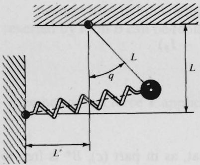
Figure P9.11

The generalized active force F corresponding to q can be expressed as

F=m g L\sum_{i=1}^{\infty}b_{i}q^{i}

where b_{1} ,\,b_{2},\ldots are constants. Determine b_{1},\ b_{2} ,and b_{3} , both by using the potentialenergy V and without reference to potential energy, and comment briefy on the relative merits of the two methods.

Results \begin{array}{r}{a_{1}=0,a_{2}=3,a_{3}=0,a_{4}=\,-\frac{7}{8};b_{1}=\,-6,b_{2}=0,b_{3}=\frac{7}{2}}\end{array}

9.12 Three corners of a cube C are attached to fixed supports by means of identical, linear springs of spring constant k . When the springs are undeformed, their axes coincide with the edges of C ,as indicated in Fig. P9.12.

To bring C into a general position,the center of C is displaced to a point whose coordinates relative to fixed axes X_{1} X_{2} ， X_{3} (see Fig. P9.12) are a q_{1},\,a q_{2},\,a q_{3}

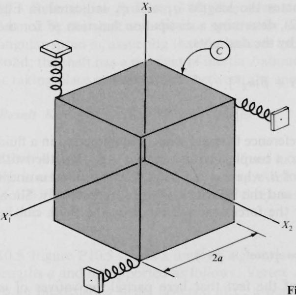
Figure P9.12

and threeaxes C_{1} C_{2} C_{3} , fixed in C and initially alignedwith X_{1} X_{2} X_{3} ,respectively, are brought into new orientations by means of successive right-handed rotationsof C of amounts q_{4} about C_{1},\,q_{5} about C_{2} , and q_{6} about C_{3}

Dropping allterms of third or higher degree in q_{i}\,(i=1,\ldots,6) ,find a potential energy contribution of the forces exerted on C by the springs.

\begin{array}{r}{\frac{1}{2}k a^{2}[(q_{1}-q_{5}-q_{6})^{2}+(q_{2}-q_{6}-q_{4})^{2}+(q_{3}-q_{4}-q_{5})^{2}]}\end{array}

9.13 Two blocks are connected to each other and to a fixed support by means of springs and dashpots, as shown in Fig. P9.13. The springs have natural lengths L_{1} and L_{2} , and the force transmitted by each dashpot is proportional to the speed of the piston relative to the cylinder, the constants of proportionality having the values \mathfrak{X} and \beta

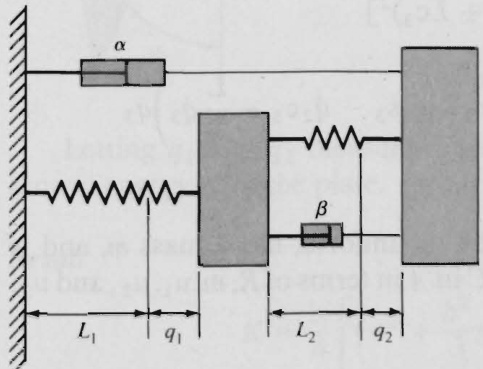
Figure P9.13

Using as generalized coordinates the lengths \pmb q_{1} and q_{2} indicated in Fig. P9.13, and letting u_{r}=\dot{q}_{r} (r=1,2) , determine a dissipation function \mathcal{F} for the set of forces exerted on the blocks by the dashpots.

Result \mathcal{F}={\textstyle\frac{1}{2}}[\alpha{u_{1}}^{2}+2\alpha u_{1}u_{2}+(\alpha+\beta){u_{2}}^{2}] \bf{*0.14} A rigid body \boldsymbol{B} moves in a reference frame \pmb{A} while \pmb{B} is immersed in a fuid that exerts on \textbf{\emph{B}} forces equivalent to a couple having a torque -\alpha\mathbf{\Gamma} , together with a force -{\boldsymbol{\beta}}\mathbf{v}, applied at a point P of \boldsymbol{B} , where \pmb{\alpha} and \beta are constants, and \mathbf{\delta}^{\mathbf{\omega}} and \mathbf{v} are the angular velocity of \pmb{B} in A and the velocity of \pmb{P} in \pmb{A} ,respectively. Show that {\mathcal{F}}, a dissipation function for the forces exerted on \pmb{B} by the fluid, can be expressed as

\mathcal{F}=\textstyle\frac{1}{2}(\alpha\pmb{\omega}^{2}+\beta\pmb{\mathrm{v}}^{2})

Suggestion: Take advantage of the fact that here partial derivatives of \pmb{\omega} with respect to generalized speeds are partial angular velocities of \textbf{\emph{B}} [seeEqs. (2.14.1)]; a similar statement applies to partial derivatives of v and partial velocities of P [see Eqs. (2.14.2)].

PROBLEM SET 10

(Secs. 5.4-5.6)

10.1 Referring to the example in Sec. 2.9, and letting \boldsymbol{P}_{1} and P_{2} have masses m_{1} and m_{2} , respectively, express the kinetic energies ^{A}K^{s} and \pmb{{\cal B}}\pmb{{\cal K}}^{s} of s in \pmb{A} and \pmb{B}. respectively, in terms of m_{1},\,m_{2},\,L,\,\omega,\,q_{1},\,q_{2},\,q_{3} , and the first time-derivatives of q_{1},q_{2},q_{3} , the generalized coordinates shown in Fig. 2.10.1.

Results

\begin{array}{l}{{^{A}{K^{S}}=\,^{B}\!K^{S}+\displaystyle\frac{1}{2}\,\omega^{2}\big[m_{1}{q_{1}}^{2}+m_{2}(q_{1}+L{\bf c}_{3})^{2}\big]\quad\quad\quad\quad\quad\quad\quad\quad\quad\quad\quad}}\\ {{^{B}{K^{S}}=\displaystyle\frac{1}{2}\,(m_{1}+m_{2})({\dot{q}_{1}}^{2}+{\dot{q}_{2}}^{2})-m_{2}\,L\Big(\dot{q}_{1}{s}_{3}-\dot{q}_{2}{s}_{3}-\displaystyle\frac{L}{2}\,\dot{q}_{3}\Big)\dot{q}_{3}}}\end{array}

10.2 Referring to Problem 2.7, suppose that c is uniform, has a mass m , and is rolling on H_{\mathrm{~\,~}} Express the kinetic energy \pmb{K} of c in \pmb{A} in terms of R,m,u_{1},u_{2} , and \pmb{u}_{3}

Result K=(m{R^{2}}/8)({5{u_{1}}^{2}}+{u_{2}}^{2}+6{u_{3}}^{2})

10.3 Referring to Problem 3.10, determine the kinetic energy \boldsymbol{K} of the system formed by the shaft and thefour spheresfor an instant atwhich the shaft has an angular speed \omega assuming that the spheres eachhave amass m ,are uniform and solid;the shafthas amoment of inertia J about its axis; \theta=30^{\circ} ;and pure rolling is takingplace at thecontactsbetween the spheres and therace R

Result K={\textstyle\frac{1}{2}}[J+18m r^{2}(2+\sqrt{3})/5]\omega^{2} \bf{*10.4} A point o of a rigid body B is fixed in a reference frame A .Show that \boldsymbol{\ K} ， the kinetic energy of B in A canbe expressed as K=K_{\omega} ,with K_{\omega} given by Eq. (5.4.3) if I denotes the inertia dyadic of B relative to o and \mathbf{w} is theangularvelocity of B in A

10.5 Figure P10.5 shows a uniform right-triangular plate of mass m and sides of lengths a and b supportedasfollows:Vertex A isfixed andvertex B is attached to an inextensible string fastened at C ,a pointvertically above A ,the length of thestringbeingsuch that line A B is horizontal.

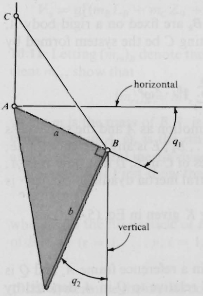
Figure P10.5

Letting q_{1} and q_{2} measure angles as indicated in Fig. P10.5, determine the kineticenergy K of theplate.

Result

K=\frac{m}{4}\Biggl[\biggl(a^{2}\,+\frac{b^{2}}{3}{\S_{2}}^{2}\biggr)\dot{q}_{1}{}^{2}\,+\,a b{\mathrm{c}}_{2}\dot{q}_{1}\dot{q}_{2}\,+\frac{b^{2}}{3}\,\dot{q}_{2}{}^{2}\Biggr]

\bf{*10.6} At a certain instant, a rigid body \pmb{B} has a rotational kinetic energy K_{\omega} and a central angular momentum \mathbf{H}. Showthat

\frac{1}{2}\frac{{\bf H}^{2}}{I_{\mathrm{max}}}\leq K_{\omega}\leq\frac{1}{2}\frac{{\bf H}^{2}}{I_{\mathrm{min}}}

where I_{\mathrm{max}} and I_{\mathrm{min}} are, respectively, the maximum and the minimum central moments of inertia of \pmb{B}

\bf{*10.7} Letting {}^{E}K^{c},{}^{E}K^{D}, and ^{A}K^{B} denote kinetic energies, show that

^{\varepsilon}K^{C}={}^{\varepsilon}K^{D}+{}^{A}K^{B}+\sum_{i=1}^{\beta}m_{i}{}^{E}\mathbf{v}^{\vec{A}_{i}}\cdot{}^{A}\mathbf{v}^{P_{i}}

if A,\,B,\,C,\,D,\,E,\,^{E}\mathbf{v}^{\overline{{A}}_{i}} and A_{\mathbf{v}}P_{i} are defined as follows: \pmb{A} , a rigid body; B_{\mathrm{:}} a set of \beta particles P_{1},...,P_{\beta} of masses m_{1},\ldots,m_{\beta} , respectively; ^{c} the system formed by \pmb{A} and B;D , a rigid body that has the_same motion as \cdot A and the same mass distribution as C;E, a reference frame; \pmb{\varepsilon}_{\mathbf{v}}\overline{{\pmb{A}}}_{i} , the velocity in \cdot E of \overline{{A}}_{i} , the point of \pmb{A} with which {\mathbf{}}P_{i} coincides; A_{\mathbf{v}}P_{i} , the velocity of P_{i} in A

\bf{*}_{10.8} The mass centers of \pmb{k} rigid bodies B_{1},\ldots,B_{k} are fixed on a rigid body \pmb{A} but B_{k} is otherwise free to move relative to A. Letting c be the system formed by \pmb{A} and B_{1},\ldots,B_{k} , show that

\ ^{\varepsilon}K^{C}={}^{\varepsilon}K^{D}+{}^{A}K^{B}+{}^{E}\!\Theta^{A}\cdot\sum_{j\,=\,1}^{k}{}\,{\bf I}^{B_{j}}\cdot{}^{A}\!\Theta^{B_{j}}

where \pmb{D} designates a rigid body that has the same motion as \pmb{A} and the same mass distribution as C;B is the set of rigid bodies B_{1},\dots,B_{k};E is any reference frame; {\varepsilon}_{K}{c} \varepsilon_{K^{D}} ^{A}K^{B} are, respectively, the kinetic energies of c in E,D in {\pmb E} and \pmb{B} in \pmb{A} \pmb{\varepsilon_{\pmb{\omega}}}_{\pmb{\omega}}^{A} is the angular velocity of \pmb{A} .n E;\mathbf{I}^{B_{j}} is the central inertia dyadic of B_{j};{^A\mathbf{\omega}_{\pmb{\omega}}^{B_{j}}} .s theangularvelocityof B_{j} in \pmb{A}

Use this result to determine the kinetic energy K given in Eq. (5.4.28)

10.9 If S is a set of \pmb{\nu} particles P_{1},\ldots,P_{v} moving in a reference frame \pmb{A} , and Q is a point moving in \pmb{A} , then the kinetic energy of s relative to Q in \pmb{A} , denoted by K^{s/Q} , is defined as

K^{S/Q}\triangleq\frac{1}{2}\sum_{i=1}^{v}m_{i}\mathbf{v}^{P_{i}/Q}

where m_{i} is the mass of \boldsymbol{P}_{i} , and \mathbf{v}^{P_{i}/Q} , called the velocity of \boldsymbol{P}_{i} relative to Q in \pmb{A} , is the difference between \mathbf{v}^{P_{i}} , the velocity of P_{i} in \pmb{A} , and \mathbf{v}^{Q} , the velocity of Q in \pmb{A} that is

\begin{array}{r l r}{{\mathbf{v}}^{P_{i}/Q}\triangleq{\mathbf{v}}^{P_{i}}-{\mathbf{v}}^{Q}}&{{}}&{(i=1,\ldots,\nu)}\end{array}

Letting s^{*} be the mass center of S, show that K^{s} , the kinetic energy of s in \pmb{A} is given by

K^{s}=K^{s/s^{*}}+K^{s^{*}}

where K^{s^{*}} is the kinetic energy in \pmb{A} of a particle whose mass is equal to the total mass of S and whose velocity in \pmb{A} is equal to the velocity of s^{*} in \pmb{A}

Comment on the relationship between these facts and Eqs. (5.4.2)-(5.4.4)

\bf{*10.10} Referring to Problem 3.15 (see also Problems 4.17, 8.14, 8.20, and 8.21), determine \pmb{K} , the kinetic energy of the robot arm in E_{\mathrm{{r}}} and V_{\gamma} , a potential energy contribution of the set of gravitational forces acting on the robot arm.

Results

\begin{array}{r l}&{K=\frac{1}{2}[A_{1}{u_{1}}^{2}+(B_{1}+C_{1}){Z_{1}}^{2}+(B_{2}+C_{2}){u_{2}}^{2}+(B_{3}+C_{3}){Z_{2}}^{2}}\\ &{\qquad+\;Z_{1}(D_{11}Z_{1}+D_{12}u_{2}+D_{13}Z_{2})+u_{2}(D_{21}Z_{1}+D_{22}u_{2}+D_{23}Z_{2})}\\ &{\quad\cdot\;+\;Z_{2}(D_{31}Z_{1}+D_{32}u_{2}+D_{33}Z_{2})+m_{A}{Z_{5}}^{2}+m_{B}(Z_{7}^{\prime}+Z_{8}^{2})}\\ &{\qquad+m_{C}({Z_{11}}^{2}+{Z_{12}}^{2}+{u_{3}}^{2})+m_{D}(Z_{17}{}^{2}+Z_{18}{}^{2}+Z_{19}{}^{2})]}\\ &{V_{\gamma}=g[(m_{B}L_{B}+m_{C}Z_{9}+m_{D}Z_{14}){s_{1}}+m_{D}p_{1}{\mathfrak c}_{1}]}\end{array}

10.11 Letting (m_{r s})_{B} denote the contribution of a rigid body \pmb{B} to the inertia coefficient m_{r s} ,showthat

(m_{r s})_{B}=m\tilde{\mathbf{v}}_{r}\cdot\tilde{\mathbf{v}}_{s}+\tilde{\mathbf{\omega}}_{r}\cdot\mathbf{I}\cdot\tilde{\mathbf{\omega}}_{s}\qquad(r,s=1,\ldots,p)

where ^{m} is the mass of B,\,\tilde{\mathbf{v}}_{r} is the rth nonholonomic partial velocity of the mass center of \pmb{B} in A,\,\tilde{\pmb{\omega}}_{r} is the rth nonholonomic partial angular velocity of \pmb{B} in \pmb{A} and I is the central inertia dyadic of \pmb{A}

Suggestion: First show that

\widetilde{\mathbf{v}}_{r}{}^{P_{i}}=\widetilde{\mathbf{v}}_{r}+\tilde{\mathbf{\omega}}\mathbf{\tilde{o}}_{r}\times\mathbf{r}_{i}

where \boldsymbol{P}_{i} is the ith particle of \pmb{B} and \mathbf{r}_{i} is the position vector from the mass center of \pmb{B} to {\mathbfcal{P}}_{i} (r=1,\ldots,p;i=1,\ldots,\nu)

10.12 Determine the inertia coefficients for the system considered in the examples in Secs. 4.8 and 5.4.

Results

\begin{array}{l}{{m_{11}=I_{A}+m_{A}a^{2}+m_{B}\left({\frac{R^{2}}{2}}+3b^{2}\right)}}\\ {{\ }}\\ {{m_{22}=m_{A}+3m_{B}}}\\ {{\ }}\\ {{m_{12}=m_{21}=0}}\end{array}

10.13 When the inertia coefficient m_{r s} differs from zero, dynamic coupling is said to exist between the generalized speeds u_{r} and u_{s}

Suppose that the mass center of a rigid body \textbf{\emph{B}} is fixed in a reference frame \pmb{A} , and let \mathbf{b}_{1},\,\mathbf{b}_{2},\,\mathbf{b}_{3} be mutually perpendicular unit vectors parallel to central principal axes of \boldsymbol{B} .Bring \textbf{\emph{B}} into a general orientation in \pmb{A} by aligning \ b_{1},\ b_{2},\ b_{3} with {\bf a}_{1},{\bf a}_{2},{\bf a}_{3} , respectively, where {\bf{a}}_{i} (i=1,2,3) is a unit vector fixed in \pmb{A} , and then subjecting \pmb{B} to successive rotations characterized by the vectors q_{1}\ b_{1},q_{2}\ b_{2} ， \boldsymbol{q}_{3}\mathbf{b}_{3} . Define generalized speeds \pmb{u}_{1} \mathbf{\psi}_{1},\;\mathbf{\psi}_{u_{2}},\;u_{3} as (a)\ u_{r}\triangleq\dot{q}_{r}\ \left(r=1,2,3\right) and (b) u_{r}\triangleq\mathbf{\omega}\cdot\mathbf{b}_{r}\,(r=1,2,3) where \mathbf{\omega} is the angular velocity of \textbf{\emph{B}} in _{A} .Determine which of the generalized speeds are coupled dynamically.

Results (a)\,u_{1} and u_{2},\,u_{1} and {u_{3}};\left(b\right) None

10.14 Referring to Problem 8.16, determine \widetilde{F}_{2}{}^{*} by using Eqs. (5.6.6). Comment briefly on the relative merits of using Eqs. (5.6.6), on the one hand, and Eqs. (4.11.1), on the other hand, to determine \widetilde{F}_{2}^{{\,\ast}}

10.15 For the system considered in Problem 8.7, determine the generalized inertia force {{F}_{1}}^{*} by using (a) Eqs. (4.11.7), (b) Eqs. (5.6.8), and (c) the formula given in Problem 8.22. Comment briefly on the relative merits of the three methods.

Result \begin{array}{r l}&{m[-29\dot{u}_{1}+19({\tt c}_{1}{\tt c}_{2}-{\tt s}_{1}{\tt s}_{2})\dot{u}_{2}-8({\tt s}_{3}{\tt s}_{1}+{\tt c}_{3}{\tt c}_{1})\dot{u}_{3}}\\ &{\quad-19({\tt s}_{2}{\tt c}_{1}+{\tt c}_{2}{\tt s}_{1})({u_{2}}^{2}/L)-8({\tt s}_{1}{\tt c}_{3}-{\tt c}_{1}{\tt s}_{3})({u_{3}}^{2}/L)]}\end{array} *_{10.16} A rigid body \pmb{B} forms a portion of a simple nonholonomic system consisting of \nu particles. Letting m be the mass, I the central inertia dyadic, \mathbf{y} the velocity of the mass center, and \mathbf{\delta}_{\mathbf{\theta}} the angular velocity of \mathbfit{B} ,show that the contribution of \textbf{\emph{B}} to the left-hand member of Eq. (5.6.1) is m\mathbf{v}\cdot\dot{\tilde{\mathbf{v}}}_{t}+\mathbf{\omega}\mathbf{\cdotI}\cdot\dot{\tilde{\mathbf{\omega}}}_{t} , where \widetilde{\mathbf{v}}_{t} and \tilde{\mathbf{o}}_{t} have the same meanings as in Eqs. (2.14.3) and (2.14.4), and the dots over these symbols denote time-differentiation in \pmb{A}

PROBLEM SET 11

(Secs. 6.1-6.3)

11.1 Referring to the example in Sec. 2.9 (see also Problems 8.1 and 8.15), let line \pmb{Y} be vertical, let P_{1} and P_{2} have masses m_{1} and m_{2} , respectively, and assume that the mass of \pmb R is negligible. Letting \pmb{A} be fixed relative to the Earth, and treating the Earth as a Newtonian reference frame, determine f_{1},f_{2} , and f_{3} such that the dynamical equations governing u_{1},u_{2} , and \pmb{u}_{3} , defined as

u_{1}\,\triangleq\,A_{\pmb{\nu}}P_{1}\cdot\mathbf{e}_{x}\qquad u_{2}\,\triangleq\,A_{\pmb{\nu}}P_{1}\cdot\mathbf{e}_{y}\qquad u_{3}\triangleq\,\dot{q}_{3}

where \pmb{\mathrm{e}}_{\pmb{x}} and \mathbf{e_{y}} are unit vectors directed as shown in Fig. 2.6.1, can be expressed as

\begin{array}{r}{\dot{u}_{i}=f_{i}\qquad(i=1,2,3)}\end{array}

Results

\begin{array}{r l}&{f_{1}=-g\mathbf{s}_{3}+\omega^{2}q_{1}\mathbf{c}_{3}+u_{2}u_{3}+({\omega^{2}}{\mathbf{c}_{3}}^{2}+{u_{3}}^{2})L m_{2}/(m_{1}+m_{2})}\\ &{f_{2}=-g\mathbf{c}_{3}-(\omega^{2}q_{1}\mathbf{s}_{3}+u_{3}u_{1})}\\ &{f_{3}=-\omega^{2}\mathbf{s}_{3}\mathbf{c}_{3}}\end{array}

11.2 For the system S formed by the particle \boldsymbol{P}_{1} , disk \pmb{D} , and rod \pmb R considered in Problems 8.2 and 8.16, make the same assumptions as in Problem 11.1 regarding the line \pmb{Y} and the reference frame \pmb{A} Determine f_{1} and f_{2} such that the dynamical equations governing u_{1} and u_{2} can be expressed as

\begin{array}{r}{\dot{u}_{i}=f_{i}\qquad(i=1,2)}\end{array}

Results

\begin{array}{l}{{f_{1}=\,-g s_{3}+\omega^{2}q_{1}\mathbf{c}_{3}+\displaystyle\frac{1}{m_{1}+m_{2}}\biggl(m_{2}L\omega^{2}{\mathbf{c}_{3}}^{2}-\frac{m_{1}}{L}\,{u_{2}}^{2}\biggr)}}\\ {{f_{2}=\,-g\mathbf{c}_{3}-\omega^{2}q_{1}\mathbf{s}_{3}+\displaystyle\frac{u_{1}u_{2}}{L}}}\end{array}

11.3 Regarding the Earth E ,Moon M , and Sun s each as a particle, let Q be the mass center of E and \pmb{S} and let F_{\varepsilon},F_{M},F_{s} and F_{Q} be reference frames in which E,M,s, and \boldsymbol{Q}_{\mathrm{:}} respectively, are fixed and whose relative orientations do not vary with time. Furthermore, assume that F_{s} can be chosen in such a way that E moves in {\pmb F}_{\pmb S} on a circular path centered at S and traced out once per year.

Assuming that F_{Q} is a Newtonian reference frame, assess the advisability of regarding F_{E},\;F_{M} , and F_{s} as Newtonian reference frames for the purpose of analyzing motions of E, M, e, and m where e and m designate a low-altitude satellite of {\pmb E} and a low-altitude satellite of M , respectively. In making these assessments, assume that S,E,M,\epsilon , and m are at all times coplanar, and let the distances and angular speeds indicated in Fig. P11.3 have the following values:

\begin{array}{r l}{{R_{S Q}}=4.5\,\times\,10^{5}\mathrm{~m~}}&{{}\quad{R_{Q E}}=\mathrm{~1.5~}\times\,10^{11}\mathrm{~m~}}\\ {{}}&{{}}\\ {{R_{E M}}=4.0\,\times\,10^{8}\mathrm{~m~}}&{{}\quad{R_{E e}}=7.0\,\times\,10^{6}\mathrm{~m~}}\end{array}

R_{M m}\,=\,2.0\,\times\,10^{6}\;\mathrm{m}

\begin{array}{r l r}&{\omega_{E}=2\,\times\,10^{-\,7}\,\,\mathrm{rad/s}\;\;}&{\omega_{M}=24\,\times\,10^{-\,7}\,\,\mathrm{rad/s}}\\ &{\omega_{e}=12\,\times\,10^{-\,4}\,\,\mathrm{rad/s}\;\;}&{\omega_{m}=\,10\,\times\,10^{-\,4}\,\,\mathrm{rad/s}}\end{array}

Results Table P11.3

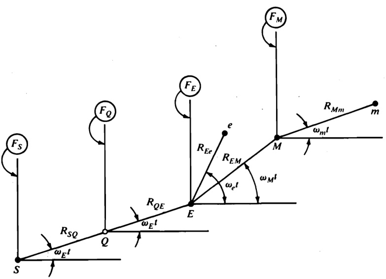
Figure P11.3

Table P11.3

<html>

Moving object	ApproximatelyNewtonian referenceframe
E	Fs
M
e	Fs Fs,FE,FM
m	Fs,FE,FM

</html>

11.4 The dynamical equations governing the generalized speeds \pmb{u}_{1} and \pmb{u}_{2} introduced in the example in Sec. 4.8 are to be formulated under the assumptions made in Problems 8.12 and 8.17. Determine f_{1} and f_{2} such that these equations can be expressed as

\begin{array}{r}{\dot{u}_{i}=f_{i}\qquad(i=1,2)}\end{array}

Results

\begin{array}{l}{{f_{1}=\displaystyle\frac{f Q_{3}+M g e\sin\theta\cos q_{1}-m_{A}a u_{1}u_{2}}{I_{A}+2J b^{2}/R^{2}+2K+m_{A}a^{2}+2m_{B}b^{2}}}}\\ {{\,}}\\ {{f_{2}=\displaystyle\frac{Q_{2}+M g\sin\theta\sin q_{1}+m_{A}a u_{1}}{m_{A}+2m_{B}+2J/R^{2}}^{2}}.}\end{array}

where

\begin{array}{l}{{Q_{2}=\cfrac{-\mu^{\prime}u_{2}Q_{1}}{{\left({u_{2}}^{2}\right.+\left.f^{2}u_{1}^{\ 2}\right)}^{1/2}}}}\\ {{\phantom{Q_{2}=}Q_{3}=\cfrac{-\mu^{\prime}u_{1}f Q_{1}}{{\left({u_{2}}^{2}\right.+\left.f^{2}u_{1}^{\ 2}\right)}^{1/2}}}}\end{array}

with

Q_{1}=\frac{e M g\cos{\theta}}{f-\mu^{\prime}R u_{2}/({u_{2}}^{2}+f^{2}{u_{1}}^{2})^{1/2}}

11.5 Referring to Problem 2.7 and letting c be a uniform disk rolling on \pmb{H} determine f_{1},f_{2} , and f_{3} such that the dynamical equations governing u_{1},\,u_{2} ,and \pmb{u}_{3} as defined in Problem 8.3 can be written

\begin{array}{r}{\dot{u}_{i}=f_{i}\qquad(i=1,2,3)}\end{array}

Results

\begin{array}{r l}&{f_{1}=\frac{1}{5}(u_{2}^{~2}\tan q_{2}-6u_{2}u_{3}-4g\mathrm{s}_{2}/R)}\\ &{f_{2}=2u_{3}u_{1}-u_{1}u_{2}\tan q_{2}}\\ &{f_{3}=\frac{2}{3}u_{1}u_{2}}\\ &{\mathrm{~\\\\\}}\\ &{\mathrm{~\\\\}.}\end{array}

11.6 A couple of torque T\mathbf{a}_{z} is applied to the link of length L_{1} of Problem 4.3. Determine f_{1} such that the dynamical equation governing \pmb{u}_{1} as defined in Problem 8.6 can be written \dot{u}_{1}=f_{1}

Result

\begin{array}{r l}&{f_{1}=\Bigg\{[T+(\tilde{F}_{1})_{\gamma}]\sin^{2}(q_{2}-q_{3})}\\ &{\qquad+\;m_{2}L_{1}L_{3}\sin(q_{1}-q_{2})\Bigg[\frac{L_{1}}{L_{3}}u_{1}(u_{2}-u_{1})\cos(q_{1}-q_{2})}\\ &{\qquad+\;u_{3}(u_{3}-u_{2})\cos(q_{2}-q_{3})\Bigg]\Bigg\}/\Bigg\{\Bigg[m_{1}\sin^{2}(q_{3}-q_{2})}\\ &{\qquad+\;m_{2}\sin^{2}(q_{1}-q_{2})\Bigg]L_{1}\Bigg\}}\end{array}

where (\tilde{F}_{1})_{\gamma} is the generalized active force contribution found in Problem 8.6.

\bf{*}_{11.7} Referring to Problem 3.15 (see also Problems 4.17, 8.14, 8.20, 8.21 and 10.10), show that the dynamical equations of motion of the robot arm can be expressedas

\sum_{r\,=\,1}^{3}\,X_{s r}\dot{u}_{r}=\,Y_{s}\qquad(s\,=\,1,2,3)

where X_{r s}=X_{s r}\left(r,s=1,2,3;r\neq s\right) .Determine X_{r s} and Y_{s}\left(r,s=1,2,3\right)

Results

\begin{array}{r l}&{X_{11}=-[A_{11}+c_{1}(2_{33}+Z_{41}+Z_{43})+s_{1}(Z_{39}+Z_{44}+Z_{53})+m_{s}L_{A}=^{2}}\\ &{\quad+m_{B}Z_{6}+^{2}m_{s}Z_{10}+m_{B}(Z_{13})^{2}+Z_{15})^{2}+Z_{16}\leq Z_{3}}\\ &{X_{12}=X_{21}-[Z_{31}+m_{B}(Z_{13}\Sigma_{14}-Z_{16}\rho_{1})]}\\ &{X_{13}=X_{31}-m_{B}Z_{16}}\\ &{X_{22}=-[B_{2}+C_{2}+D_{22}+m_{B}L_{B}^{2}+m_{C}Z_{9}^{2}+m_{B}(Z_{14}^{2}+P_{1}^{2})]}\\ &{X_{23}=X_{32}-m_{B}p_{1}}\\ &{X_{33}=-(m_{c}+m_{B})}\\ &{Y_{1}=\varsigma_{1}(Z_{34}+Z_{42}+Z_{33})+s_{1}(Z_{40}+Z_{43}+Z_{34})+m_{B}Z_{6}Z_{32}}\\ &{\quad+m_{C}Z_{10}Z_{27}+m_{B}(Z_{13}\Sigma_{32}+Z_{15}Z_{33}+Z_{16}Z_{34})-T_{1}\varepsilon^{2}}\\ &{Y_{2}=Z_{38}+Z_{43}+Z_{52}+m_{B}L_{B}Z_{12}+m_{C}Z_{26}+m_{B}(Z_{14}Z_{32}-p_{1}Z_{34})}\\ &{\quad-T_{24}\varepsilon^{3}+g[(m_{B}L_{B}+m_{C}Z_{9}+m_{B}Z_{14})\varepsilon_{1}-m_{B}\varepsilon_{2}}\\ &{Y_{3}=m_{B}Z_{28}+m_{B}Z_{34}-K_{1}\varepsilon^{4}+g(m_{A}+m_{B})\mathfrak{I}_{3}}\end{array}

\bf{*}_{11.8} Referring to Problem 3.15 (see also Problems 4.17, 8.14, 8.20, 8.21, 10.10, and 11.7), suppose that D^{*} lies on line B^{\ast}C^{\ast} and that each central principal axis of \textbf{\emph{D}} is parallel to one of \mathbf{b}_{1},\mathbf{b}_{2},\mathbf{b}_{3} . Show that under these circumstances the dynamical equations of motion reduce to

\dot{u}_{r}=\frac{Y_{r}}{X_{r r}}\qquad(r=1,2,3)

\bf{*}\bf{11.9} Show that Eqs. (6.1.1) can be written

F_{r}+F_{r}^{\;\ast}+\sum_{\substack{s=\,p+1}}^{n}\,(F_{s}+F_{s}^{\;\ast})A_{s r}=0\qquad(r=1,\ldots,p)

where F_{1},\ldots,F_{n} are holonomic generalized active forces for s in N,F_{1}{}^{*},\ldots,F_{n}{}^{*} are holonomic generalized inertia forces for s in N and A_{p+1,\,1},\dotsc,A_{n,\,p} have the same meaning as in Eqs. (2.13.1).

11.10 Figure P11.10 represents a one-cylinder reciprocating engine consisting ofacounter-weightedcrank A , connecting rod B ,piston C ,and cylinder D A^{*},B^{*} and C^{*} are the mass centers of A B and C ,respectively,and A,\,B and C have masses m_{A} ， m_{B} , and m_{C} ,respectively.The central radii of gyration of A and B withrespect toaxesnormal tothemiddleplaneofthemechanismhavethe values k_{A} and k_{B} , respectively.

The system s formed by A,\,B and C possesses one degree of freedom in a reference frame in which point o and the axis of the cylinder are fixed; the angle q_{1} shown in Fig. P11.10, and u_{1} defined as u_{1}\triangleq\dot{q}_{1} , can serve, respectively, as a generalized coordinate and as a generalized speed associated with this degree of freedom. However, it can be convenient, for example,for the purpose of bringing certain interaction forces into evidence（see Sec. 4.9), to introduce additionai generalized speeds, u_{2} and u_{3} ,as

u_{2}\triangleq{\mathbf{\omega}}\mathbf{\omega}^{B}\cdot\mathbf{n}_{2}\qquad u_{3}\triangleq\mathbf{\omega}\mathbf{v}^{C^{\ast}}\cdot\mathbf{n}_{3}

Moreover, it is then helpful to define, in addition, an angle q_{2} as indicated in Fig.
P11.10.

Letthesetofcontactforcesexertedon A by thecrankshafton which A is mounted be equivalent to a couple of torque \alpha_{1}\mathbf{n}_{1}+\alpha_{2}\mathbf{n}_{2}+\alpha_{3}\mathbf{n}_{3} ,together with a force P_{1}\mathbf{n}_{1}+P_{2}\,\mathbf{n}_{2}+P_{3}\,\mathbf{n}_{3} applied at o ,and let the set of contact forces exerted on C by exploding gases and by the cylinder D be equivalent to a couple of torque \beta_{1}\mathbf{n}_{1}+\beta_{2}\mathbf{n}_{2}+\beta_{3}\mathbf{n}_{3} , together with a force Q_{1}\mathbf{n}_{1}+Q_{2}\mathbf{n}_{2}+Q_{3}\mathbf{n}_{3} applied at \zeta^{*} Finally, let the set of forces exerted by B on A be equivalent to a couple of torque \gamma_{1}\mathbf{n}_{1}+\gamma_{3}\mathbf{n}_{3} , together with a force R_{1}\mathbf{n}_{1}+R_{2}\mathbf{n}_{2}+R_{3}\mathbf{n}_{3} applied at point P

After verifying that u_{2} and \boldsymbol{u}_{3} must satisfy the motion constraint equations

\begin{array}{l}{{\displaystyle{u_{2}=-\,\frac{a{\bf c}_{1}}{b{\bf c}_{2}}\,u_{1}}}}\\ {{\displaystyle{u_{3}=\,-\,\frac{a}{\bf c}_{2}\,({\bf s}_{1}{\bf c}_{2}+{\bf c}_{1}{\bf s}_{2})u_{1}}}}\end{array}

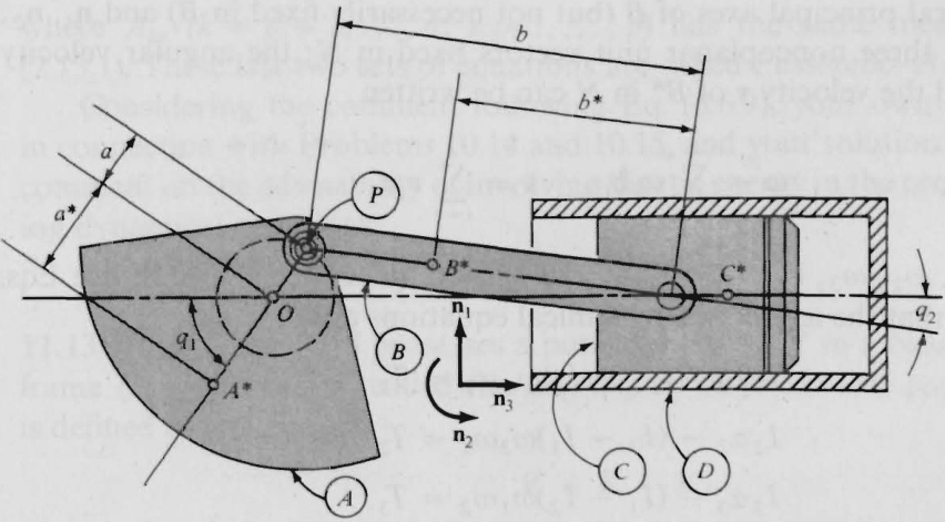
Figure P11.10

write dynamical equations governing all motions of \boldsymbol{s}\left(\boldsymbol{a}\right) by using Eqs. (6.1.2) with r=1 , 2, 3 and (b) by using the equation in Problem 11.9 with p=1 . Neglect gravitational forces, and verify that the result of part (b) can be obtained from those of part (a) by using the first two equations of part (a) to eliminate R_{3} from the third equation.

Results

m_{A}[(a^{*})^{2}\,+\,{k_{A}}^{2}]\dot{u}_{1}=\alpha_{2}\,+\,a(R_{1}\mathbf{c}_{1}\,-\,R_{3}\mathbf{s}_{1})

m_{B}\{[(b^{*})^{2}\,+\,k_{B}^{\,\,2}]\dot{u}_{2}\,-\,b^{*}s_{2}\,\dot{u}_{3}\}=b(R_{1}\mathrm{c}_{2}\,+\,R_{3}\mathrm{s}_{2})

(m_{B}+m_{C})\dot{u}_{3}-m_{B}b^{*}s_{2}\,\dot{u}_{2}=Q_{3}-R_{3}-m_{B}b^{*}{\bf c}_{2}\,u_{2}^{\;2}

(b)\ m_{A}[(a^{*})^{2}+k_{A}{}^{2}]\dot{u}_{1}+\frac{m_{B}a}{\mathtt{c}_{2}}\biggl\langle\biggl\{b^{*}\mathtt{s}_{2}(\mathtt{s}_{1}\mathtt{c}_{2}+\mathtt{c}_{1}\mathtt{s}_{2})-\mathtt{c}_{1}\biggl[\frac{(b^{*})^{2}+k_{B}{}^{2}}{b}\biggr]\biggr\}\dot{u}_{2}

\begin{array}{r l}&{+\,\biggl[-\cfrac{m_{C}}{m_{B}}\,(\mathsf{s}_{1}\mathsf{c}_{2}+\mathsf{c}_{1}\mathsf{s}_{2})+\Big(\cfrac{b^{*}}{b}-1\Big)\mathsf{c}_{1}\mathsf{s}_{2}-\mathsf{s}_{1}\mathsf{c}_{2}\biggr]\dot{u}_{3}\biggr\}}\\ &{=\alpha_{2}+\,a(\mathsf{s}_{1}\mathsf{c}_{2}+\mathsf{c}_{1}\mathsf{s}_{2})\bigg(m_{B}{b^{*}}{u_{2}}^{2}-\cfrac{Q_{3}}{\mathsf{c}_{2}}\bigg)}\end{array}

11.11 When a rigid body \textbf{\emph{B}} moves in a Newtonian reference frame N under the action of a set of contact and distance forces equivalent to a couple of torque \mathbf{T} together with a force \mathbf{F} applied at the mass center B^{*} of \pmb{B} , the vectors \mathbf{T} and \mathbf{F} always can be expressed as

\mathbf{T}=\sum_{i=1}^{3}\,T_{i}\mathbf{b}_{i}\qquad\mathbf{F}=\sum_{i=1}^{3}\,F_{i}\mathbf{n}_{i}

where \ensuremath{\mathbf{b}}_{1},\,\ensuremath{\mathbf{b}}_{2} , and {\bf b}_{3} form a dextral set of mutually perpendicular unit vectors parallel to central principal axes of \textbf{\emph{B}} (but not necessarily fixed in \textbf{\emph{B}} ) and \mathbf{u}_{1},\mathbf{n}_{2} and \mathbb{n}_{3} are any three noncoplanar unit vectors fixed in N ; the angular velocity \mathbf{\delta}_{\mathbf{\delta}}^{\mathbf{\alpha}} of \textbf{\emph{B}} in N and the velocity \mathbf{v} of B^{*} in N can be written

\mathbf{\omega}\Leftrightarrow\sum_{i=1}^{3}\omega_{i}\mathbf{b}_{i}\qquad\mathbf{v}=\sum_{i=1}^{3}v_{i}\mathbf{n}_{i}

Letting \omega_{1},\,\omega_{2},\,\omega_{3},\,v_{1},\,v_{2},\,v_{3} play the roles of generalized speeds, use Eqs. (6.1.2) to show that the associated dynamical equations are

\begin{array}{r}{I_{1}\boldsymbol{\alpha}_{1}-(I_{2}-I_{3})\boldsymbol{\omega}_{2}\boldsymbol{\omega}_{3}=T_{1}}\\ {I_{2}\boldsymbol{\alpha}_{2}-(I_{3}-I_{1})\boldsymbol{\omega}_{3}\boldsymbol{\omega}_{1}=T_{2}}\\ {I_{3}\boldsymbol{\alpha}_{3}-(I_{1}-I_{2})\boldsymbol{\omega}_{1}\boldsymbol{\omega}_{2}=T_{3}}\end{array}

F_{1}=m\dot{v}_{1}\qquad F_{2}=m\dot{v}_{2}\qquad F_{3}=m\dot{v}_{3}

where I_{j} is the moment of inertia of \pmb{B} about a line passing through B^{*} and parallel to \mathbf{b}_{i} , and \alpha_{i}\triangleq\,\alpha\cdot\mathfrak{b}_{i} ,with \pmb{\upalpha} the angular acceleration of \boldsymbol{B} in N Thefirstthree equations are known as Euler's dynamical equations, and the last three equations express Newton's second law of motion for the mass center of a rigid body.

11.12 Referring to Sec. 5.6, show that one can use Eqs. (6.1.1) or Eqs. (6.1.2) to generate dynamical equations involving the kinetic energy K of asystem s ina Newtonian reference frame, as follows.

For a holonomic systemwith u_{r}\,\triangleq\,{\dot{q}}_{r}\,(r=1,\dots,n),

{\frac{d}{d t}}\;{\frac{\partial K}{\partial{\dot{q}}_{r}}}-{\frac{\partial K}{\partial q_{r}}}=F_{r}\;\;\;\;\;\;\;(r=1,\ldots,n)

These equations are known as Lagrange's equations of the first kind.

For a holonomic system with u_{\nu} defined as in Eqs. (2.12.1), so that Eqs. (2.14.5) apply,

\sum_{s=1}^{n}\bigg(\frac{d}{d t}\frac{\partial K}{\partial\dot{q}_{s}}-\frac{\partial K}{\partial q_{s}}\bigg)W_{s r}=F_{r}\,\,\,\,\,\,\,\,\,\,\,(r=1,\ldots,n)

For a nonholonomic system with u_{r}\,\triangleq\,{\dot{q}}_{r}\,(r=1,\dots,n)

\frac{d}{d t}\frac{\partial K}{\partial{\dot{q}}_{r}}-\frac{\partial K}{\partial q_{r}}+\sum_{\substack{s=p+1}}^{n}\bigg(\frac{d}{d t}\frac{\partial K}{\partial{\dot{q}}_{s}}-\frac{\partial K}{\partial q_{s}}\bigg)C_{s r}={\widetilde F}_{r}\qquad(r=1,\ldots,p)

where C_{s r}\left(s=p+1,\ldots,n;r=1,\ldots,p\right) has the same meaning as in Eqs. (5.1.13). For a nonholonomic system with u_{r} defined as in Eqs. (2.12.1), so that Eqs. (2.14.5) apply,

\sum_{s=1}^{n}\left({\frac{d}{d t}}{\frac{\partial K}{\partial{\dot{q}}_{s}}}-{\frac{\partial K}{\partial q_{s}}}\right)\left(W_{s r}\,+\,\sum_{k=\,p+1}^{n}\,W_{s k}\,A_{k r}\right)={\widetilde F},\qquad(r=1,\ldots,p)

where A_{k r} {\bf\Psi}_{k r}\;\left(k=p+1,\ldots,n;\;r=1,\ldots,p\right) has the same meaning as in Eqs.
(2.13.1). These last two sets of equations are called Passerello-Huston equations.

Considering the comment following Eq. (5.6.9), your own comments made in connection with Problems 10.14 and 10.15, and your solution of Problem 4.18, comment on the advisability of involving kinetic energy in the process of formulating dynamical equations.

11.13 When a system S possesses a potential energy \pmb{V} in a Newtonian reference frame N a quantity \mathcal{L}, called the Lagrangian or the kinetic potential of \pmb{S} in N is defined as

{\mathcal{L}}\triangleq K-V

where \pmb{K} is the kinetic energy of s in N

Supposing that \boldsymbol{s} is a holonomic system with generalized speeds defined as u_{r}\triangleq\dot{q}_{r} (r=1,\ldots,n) , where q_{1},\ldots,q_{n} are generalized coordinates for \boldsymbol{s} in N show that \mathcal{L}, . regarded as a function of q_{1},\ldots,q_{n},\;\dot{q}_{1},\ldots,\dot{q}_{n}, and the time t_{\mathrm{:}} satisfies the equations

\frac{d}{d t}\frac{\partial\mathcal{L}}{\partial\dot{q}_{r}}-\frac{\partial\mathcal{L}}{\partial q_{r}}=0\qquad(r=1,\ldots,n)

These equations are called Lagrange's equations of the second kind.

11.14 Referring to the example in Sec. 4.8 (see also Problems 8.12 and 8.17) express Q_{1} as a function of \mu^{\prime},R,M,g,e,f,\theta,u_{1}, and \pmb{u}_{2}

\lambda_{1}=e M g\cos{\theta}/[f-\mu^{\prime}R u_{2}/({u_{2}}^{2}+f^{2}{u_{1}}^{2})^{1/2}]

PROBLEM SET 12

(Secs. 6.4-6.7)

12.1 Referring to the discussion in Sec. 6.4 of motions of the bar \pmb{B} depicted in Fig. 6.4.3, suppose that h=3R/4 and \Omega^{2}=2g/R . Find a value of \bar{\pmb q}_{1} other than zero such that the equation q_{1}=\bar{q}_{1} describes a possible motion of \pmb{B} , and determine N such that the circular frequency of small amplitude oscillations of \pmb{B} that ensue subsequent to a small disturbance of this motion is equal to N(g/R)^{1/2}

\bar{q}_{1}=\cos^{-\,1}(9/10)\qquad N=(19/85)^{1/2}

12.2 In Fig. P12.2, A,\,B, and c are the outer gimbal, the inner gimbal, and the rotor of a gyroscope, and P is a particle of mass m attached to the rotor axis at a distance \pmb{h} from the center of c . By means of an electric motor (not shown) that may be regarded as consisting of two parts, one rigidly attached to \pmb{B} , the other to C,C is driven relative to \pmb{B} in such a way that the angular velocity of c in \pmb{B} is given by

{\bf\mathcal{B}}_{\bf60}{\bf\mathcal{C}}=s{\bf b}_{1}

where s is a constant and {\bf b_{1}} is a unit vector directed as shown. The inertia properties of A,B, and c are characterized by the five quantities I,J_{1},J_{2},K_{1} and K_{2} defined in terms of the central inertia dyadics \mathbf{I}_{A},\mathbf{I}_{B} , and \mathbf{I}_{c} of A,B, and c , respectively, as follows:

I\triangleq\mathbf{a}_{1}\cdot\mathbf{I}_{A}\cdot\mathbf{a}_{1}\qquad J_{r}\triangleq\mathbf{b}_{r}\cdot\mathbf{I}_{B}\cdot\mathbf{b}_{r}\qquad K_{r}\triangleq\mathbf{b}_{r}\cdot\mathbf{I}_{C}\cdot\mathbf{b}_{r}\qquad(r=1,2)

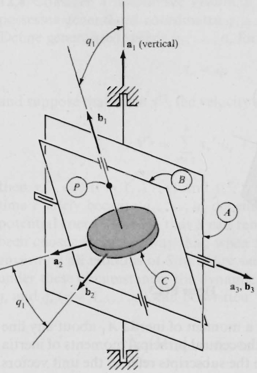
Figure P12.2

where {\bf a}_{1} and {\bf b}_{2} are unit vectors directed as shown, and {\bf b}_{1} {\bf b}_{2} ,and {\bf b}_{3}\triangleq{\bf b}_{1}\times{\bf b}_{2} are parallel to central principal axes of both B and C Moreover, {\bf b}_{3}\cdot{\bf I}_{B}\cdot{\bf b}_{3}= J_{1} and {\bf b}_{3}\cdot{\bf I}_{C}\cdot{\bf b}_{3}=K_{2}

The system formed by A,B,C ,and P can move in such a way that q_{1} ,the angle between \mathbf{a}_{1} and {\bf b}_{1} , remains equal to zero while the angular velocity of A is given by

\mathbf{\Theta}\mathbf{o}^{A}=p\mathbf{a}_{1}

where p is a constant. Letting {q_{1}}^{*} be aperturbation of q_{1} ,determine \omega^{2} suchthat {q_{1}}^{*} is governed by the (linearized) differential equation

\ddot{q}_{1}{}^{*}+\omega^{2}{q_{1}}^{*}\approx0

Result

\omega^{2}=\frac{p[p(J_{1}+K_{1}-J_{2}-K_{2}-m h^{2})+s K_{1}]-m g h}{J_{1}+K_{2}+m h^{2}}

12.3 The system S depicted in Fig. P12.3 consists of a rod A of mass m_{A} ,one end of which is pinned to a fixed support at a point o while the other end supports a uniform plate B of mass m_{B} in such a way that B can rotate freely about the axis of A The distances from o to A^{*} and B^{*} , the mass centers of A and B ,respectively, are L_{A} and L_{B} , respectively. Finally, A has a moment of inertia A_{1} about any line normal to A and passing through A^{*} , and the central principal moments of inertia B have the values B_{1} B_{2} ,and B_{3} , where the subscripts refer to the unit vectors \mathbf{b}_{1},\,\mathbf{b}_{2} , and {\bf b}_{3} shown in Fig. P12.3.

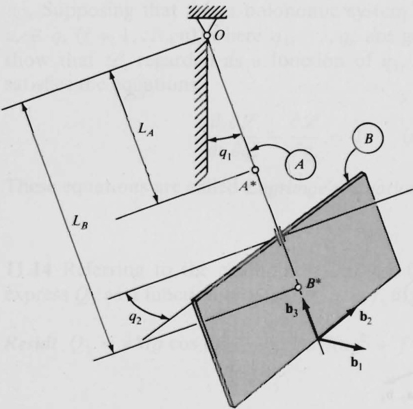
Figure P12.3

s can move in such a way that the angles q_{1} and q_{2} (see Fig. P12.3) are given for all values of the time t by

q_{1}={\tilde{q}}_{1}\qquad q_{2}=0

where \tilde{q}_{1} is a function of t Letting {q_{1}}^{*} and {q_{2}}^{*} be perturbations such that

q_{1}=\tilde{q}_{1}+q_{1}^{~*}~~~~~~q_{2}=q_{2}^{~*}

formulate differential equations linearized in q_{1}{}^{*},\,q_{2}{}^{*},\,\dot{q}_{1}{}^{*} and {{\dot{q}}_{2}}^{*} Use these equations to verify that \tilde{q}_{1},\,q_{1}^{\mathrm{~\*~}} and {q_{2}}^{*} satisfy the differential equations

\ddot{\tilde{q}}_{1}+\alpha\sin{\tilde{q}_{1}}\approx0

\ddot{q}_{1}^{~*}+\alpha\cos\tilde{q}_{1}q_{1}^{~*}\approx0\qquad\ddot{q}_{2}^{~*}-\beta\dot{\tilde{q}}_{1}^{~2}q_{2}^{~*}\approx0

where \boldsymbol{\mathfrak{x}} and \beta are constants, and determine these constants. Answer the following questionsregarding the differential equations: (a) Are all of the equations linear differential equations? \mathit(b) Are the last two equations linear differential equations? (c) Is one or more of the equations a differential equation with constant coefficients? (d) Are the last two equations differential equations with constant coefficients?

Results

\alpha={\frac{g(m_{A}L_{A}+m_{B}L_{B})}{A_{1}+B_{1}+m_{A}{L_{A}}^{2}+m_{B}{L_{B}}^{2}}}\qquad\beta={\frac{B_{2}-B_{1}}{B_{3}}}

12.4 Consider a holonomic system S that consists of particles P_{1},...,P_{\nu} and possesses generalized coordinates q_{1},\ldots,q_{n} in a Newtonian reference frame N Define generalized speeds u_{1},\ldots,u_{n} for s in N as

u_{r}=\dot{q}_{r}\qquad(r=1,\dots,n)

and suppose that when \mathbf{v}^{P_{i}} , the velocity of P_{i} in N , is expressed as [see Eq. (2.14.2)]

\mathsf{v}^{P_{i}}=\sum_{r=1}^{n}\mathsf{v}_{r}^{P_{i}}u_{r}+\mathsf{v}_{t}^{\ P_{i}}\qquad(i=1,\ldots,\nu)

then \mathbf{v}_{t}^{\,P_{i}}=0\ (i=1,\dots,\nu) and \mathbf{v}_{r}^{~P_{i}}~(i=1,\ldots,{\nu};\,r=1,\ldots,{n}) depends on the time t solely because q_{1},\ldots,q_{n} depend on t. Finally, assume that s possesses a potential energy V in N , that s can remain at rest in N , and that q_{1},\ldots,q_{n} have been chosen in such a way that, when s is at rest in N , the dynamical equations governing all motions of s in N are satisfied by q_{r}\equiv0\,(r=1,\dots,n) .Show that under these. circumstances the dynamical equations of s in N , when linearized in q_{r} and {\dot{q}}_{r}\left(r=1,\dots,n\right) , can be written

\sum_{s\,=\,1}^{n}\,(M_{r s}\ddot{q}_{s}\,+\,K_{r s}q_{s})\approx0\qquad(r\,=\,1,\ldots,n)

where M_{r s} (r,s=1,\ldots,n) are the values of the inertia coefficients of \boldsymbol{s} in N (see Sec. 5.5) when q_{1}=\cdots=q_{n}=0, and K_{r s} denotes the value of \partial^{2}V/\partial q_{r}\,\partial q_{s} (r,s=1,\ldots,n) when q_{1}=\cdots=q_{n}=0.

Suggestion: Refer to Eq. (5.1.2) for F_{\mathrm{,}} ， (r=1,\ldots,n) , and make use of the facts that

{\frac{\partial V}{\partial q_{r}}}={\frac{\partial V(0)}{\partial q_{r}}}+\sum_{s=1}^{n}{\frac{\partial^{2}V(0)}{\partial q_{r}\,\partial q_{s}}}q_{s}+\,\cdots\qquad(r=1,\ldots,n)

while

\boldsymbol{\mathsf{v}}_{r}^{\,P_{i}}=\boldsymbol{\mathsf{v}}_{r}^{\,P_{i}}(0)\,+\,\sum_{s=1}^{n}\frac{\partial\boldsymbol{\mathsf{v}}_{r}^{\,P_{i}}(0)}{\partial q_{s}}\,q_{s}\,+\,\cdots\qquad(i=1,\ldots,\nu;r=1,\ldots,n)

from which it follows that the linearized velocity of P_{i} is given by

\mathbf{v}^{P_{i}}\approx\sum_{r=1}^{n}\mathbf{v}_{r}{}^{P_{i}}(0)\dot{q}_{r}\qquad(i=1,\ldots,\nu)

\bf{*}_{12.5} Referring to Problem 9.9, letting \pmb{A} be a Newtonian reference frame, and using as generalized speeds for \boldsymbol{B} in \pmb{A} the quantities {\dot{q}}_{1},{\dot{q}}_{2} , and \dot{\boldsymbol{q}}_{3} , form linearized dynamical equations governing q_{1},\,q_{2},\,q_{3} . Do this by employing the result developed in Problem 12.4.

Result

\begin{array}{c}{{\ddot{q}_{1}\approx0}}\\ {{\ddot{q}_{2}+3G m\displaystyle\frac{I_{3}-I_{1}}{I_{2}R^{3}}~q_{2}\approx0}}\\ {{.}}\\ {{\ddot{q}_{3}-3G m\displaystyle\frac{I_{1}-I_{2}}{I_{3}R^{3}}q_{3}\approx0}}\end{array}

12.6 Two uniform bars, B_{1} and B_{2} , each of length L and mass m , are supported by pins, as indicated in Fig. P12.6, and are attached to each other by a light, linear spring of natural length L/4 and spring constant mg/ \boldsymbol{L} Formulate equations that govern the angles q_{1} and q_{2} (see Fig. P12.6) when B_{1} and B_{2} are at rest, and verify that two sets of values satisfying these equations are q_{1}=35.55^{\circ} q_{2}=44.91^{\circ} and q_{1}=-114.69^{\circ}, q_{2}=\mathrm{~-}94.77^{\circ}

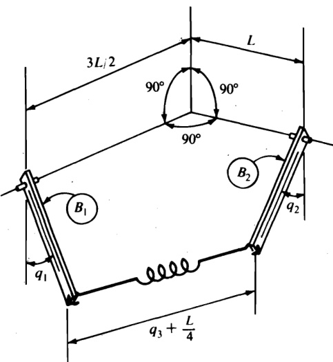
Figure P12.6

Suggestion: Introduce the stretch of the spring as a pseudo-generalized coordinate \pmb q_{3} that must satisfy the configuration constraint equation

\left(q_{3}+\frac{L}{4}\right)^{2}=L^{2}\biggl[(1-{\bf s}_{1})^{2}+\left(\frac{3}{2}-{\bf s}_{2}\right)^{2}+({\bf c}_{1}-{\bf c}_{2})^{2}\biggr]

After defining generalized speeds u_{1},u_{2} , and u_{3}\left(u_{3}\right) is a pseudo-generalized speed) as

u_{r}\triangleq\dot{q}_{r}\qquad(r=1,2,3)

and diferentiating the configuration constraint equation to obtain a motion constraint equation having the form of Eqs. (5.1.13), use Eqs. (6.5.4).

Results

\begin{array}{c}{{\displaystyle{\left(\frac{q_{3}}{L}+\frac{1}{4}\right)\!s_{1}+2\frac{q_{3}}{L}\left(\mathtt{c}_{2}\mathtt{s}_{1}-\mathtt{c}_{1}\right)=0}}}\\ {{\displaystyle{\left(\frac{q_{3}}{L}+\frac{1}{4}\right)\!\mathtt{s}_{2}+2\frac{q_{3}}{L}\left(\mathtt{c}_{1}\mathtt{s}_{2}-\frac{3}{2}\mathtt{c}_{2}\right)=0}}}\end{array}

12.7 Two particles, \boldsymbol{P}_{1} and P_{2} , of masses m_{1} and m_{2} , respectively, are supported by a light linkage, as indicated in Fig. P8.6, where \mathbf{a}_{\mathbf{x}} and a, are unit vectors directed vertically downward and horizontally, respectively. Assuming that this system is at rest, verify that the parameters L_{1},L_{2},L_{3},L_{4},m_{1}, and m_{2} are related to the variables q_{1},q_{2} , and q_{3} as follows:

\begin{array}{r}{L_{1}\mathbf{c}_{1}+L_{2}\mathbf{c}_{2}-L_{3}\mathbf{c}_{3}=0}\\ {L_{1}\mathbf{s}_{1}+L_{2}\mathbf{s}_{2}-L_{3}\mathbf{s}_{3}-L_{4}=0}\\ {m_{1}\mathbf{s}_{1}+m_{2}\mathbf{s}_{3}\displaystyle\frac{\sin(q_{2}-q_{1})}{\sin(q_{2}-q_{3})}=0}\end{array}

12.8 Referring to Problem 8.7, formulate three equations relating Q,\,R,\,S,\,q_{1}, q_{2},q_{3} ,and m when all rods are at rest.

Result

\begin{array}{r}{(-Q+R+S)\mathbf{c}_{1}-30m g\mathbf{s}_{1}=0}\\ {(Q-R)\mathbf{c}_{2}-19m g\mathbf{s}_{2}=0}\\ {R\mathbf{c}_{3}-8m g\mathbf{s}_{3}=0}\end{array}

\pmb{*12.9} Referring to Problem 8.10, formulate an equation relating T_{B} to T_{E} when B,C,C^{\prime},D,D^{\prime},E, and {\pmb F} are atrest.

Result T_{B}+244T_{E}=0

12.10 Referring to Problem 3.11, and letting T\mathbf{N},\,T^{\prime}\mathbf{N} , and tn be the torques of couples applied to A,\,A^{\prime} , and \pmb{D} , respectively show that T,\,T^{\prime} and \boldsymbol{t} satisfy the equations

T=T^{\prime}=-\,{\frac{t a}{2d}}

when the system is at rest.

12.11 Figure P12.11 shows four bars, each of length L , connected by hinges and linear springs, the springs having spring constants k_{\textrm{1}} and k_{2} and equal natural lengths L/2 . Neglecting gravitational effects, show that when this system is at rest,then

\frac{k_{1}}{k_{2}}=\frac{1-\frac{1}{2}[2(1-\cos q)]^{-1/2}}{1-\frac{1}{2}[2(1+\cos q)]^{-1/2}}

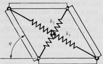
Figure P12.11

12.12 Referring to Problem 12.2, consider the steady motion characterized by theequations

q_{1}=\bar{q}_{1}\qquad{\mathbf{o}}^{A}=p{\mathbf{a}}_{1}

where \bar{q}_{1} and p are constants. Under these circumstances, p is called the rate of precession of the gyroscope, and the motion is termed a steady precession. Determine the relationship among m,h,J_{1},J_{2},K_{1},K_{2},\bar{q}_{1},s, and p that prevails during steady precession.

p^{2}(J_{1}+K_{1}-J_{2}-K_{2}-m h^{2})\cos\bar{q}_{1}+p s K_{1}-m g h=0

12.13 In Fig.P12.13, A,\dots,E are uniform,square plates,each having a mass m and sides of length L These plates are attached to each other and to a uniform square plate F having a mass 5m and sides of length L , by means of smooth hinges.

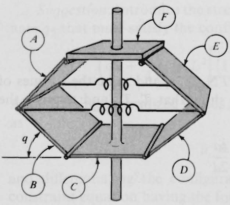
Figure P12.13

A vertical shaft, to which ^{c} is attached rigidly, passes through an opening in F thus leaving {\pmb F} free to move up and down. Finally, two light, linear springs, each having a natural length L and spring constant k_{i} . connect the plates as shown.

One possible motion of this system is the following: The shaft is made to rotate with a constant angular speed \Omega_{z} and \pmb q (see Fig. P12.13) remains constant. Showthat

\frac{L\Omega^{2}}{g}=\frac{6\cot{q}}{3\,+\,4\cos{q}}\left(4\frac{k L}{m g}\sin{q}-7\right)

under these circumstances.

PROBLEM SET 13

(Secs. 7.1-7.7)

13.1 Referring to Problem 8.6, let L_{1}=L_{4}=2\ \mathrm{m}, L_{2}=L_{3}=3\ \mathrm{m}, m_{1}=4\,{\bf k g}, m_{2}=5~\mathbf{kg} , and suppose that the system is released from rest when q_{1}=45^{\circ} Determine the value of \dot{\pmb q}_{1} for the first instant at which \pmb q_{1} vanishes.

Note: It can be verified that q_{2} and \pmb q_{3} have the values 82.281^{\circ} and 52.719^{\circ} respectively, when q_{1}=45^{\circ} , and that q_{2}=73.126^{\circ}; q_{3}=16.874^{\circ} when q_{1}=0

Result - 1.87 rad/s

13.2 Letting q_{1},\ldots,q_{n} be generalized coordinates of a holonomic system in a reference frame N , show that \pmb{H} , the Hamiltonian of \boldsymbol{s} in N (see Sec. 7.2), can be expressed as

H=\sum_{r\mathop{=}1}^{n}\frac{\partial\mathcal{L}}{\partial{\dot{q}}_{r}}{\dot{q}}_{r}-\mathcal{L}

where \mathscr{L} is the Lagrangian of s in N (see Problem 11.13), regarded as a function of q_{1},\ldots,q_{n},\dot{q}_{1},\ldots,\dot{q}_{n} , and \pmb{t}

Suggestion: Take advantage of the fact that [see Eqs. (5.5.7)-(5.5.9)] K_{0},K_{1} ? and \pmb{K}_{2} can be written, respectively, as

K_{0}=A\qquad K_{1}=\sum_{r=1}^{n}B_{r}{\dot{q}}_{r}\qquad K_{2}={\frac{1}{2}}\sum_{r=1}^{n}\sum_{s=1}^{n}C_{r s}{\dot{q}}_{r}{\dot{q}}_{s}

where A,B_{r} , and C_{r s} are independent of {\dot{q}}_{1},\dots,{\dot{q}}_{n} , and C_{r s}=C_{s r}\,(r,s=1,\ldots,n).

13.3 The axis of a circular disk \pmb{B} of radius \pmb R (see Fig. P13.3) is fixed, and \pmb{B} is made to rotate about this axis with a constant angular speed \omega .A vane \pmb{V} is fixed on \pmb{B} , the equation of the center line of V being r=R sin 2q where \boldsymbol{r} is the distance from the axis of \pmb{B} to \pmb{P} , a generic point of the center line, and \pmb q is the angle between line o P and a line o Q that is fixed on \pmb{B}. . Finally, a particle is free to move in V.

336 PROBLEM SETS

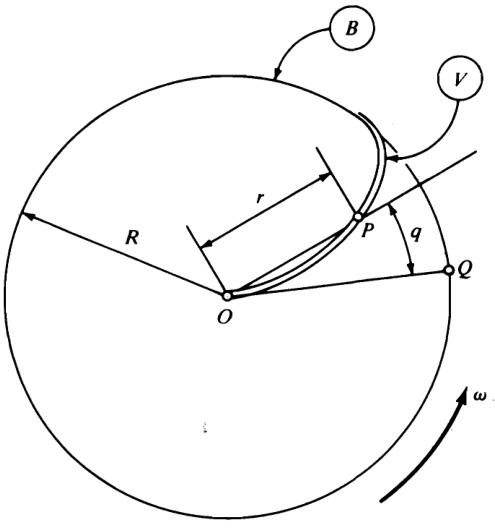
Figure P13.3

If the axis of \pmb{B} is vertical, and if the particle is inserted into V at ^o with a very small velocity (essentially zero), the particle moves toward the periphery of \pmb{B} and arrives there with a velocity having a magnitude \boldsymbol{v} .Determine \pmb{v}.

Result v=2R\omega

13.4 If the plane \pmb{H} in Problem 8.3 is perfectly smooth, the equations of motion of c possess an integral of the form

u_{2}{\bf c}_{2}+\alpha u_{3}{\bf s}_{2}=\beta

where \pmb{\alpha} is a definite constant and \beta is an arbitrary constant. Determine \pmb{\alpha}

Result \alpha=2

*_{13.5} Referring to Problem 3.15 (see also Problems 4.17, 8.14, 8.20, 8.21, 10.10, 11.7, and 11.8), determine \mathbf{H}\cdot\mathbf{a}_{1} where \mathbf{H} is the angular momentum of the robot arm in E with respect to a point on the hub axis of \bar{\pmb{A}}

Result

\begin{array}{r l}&{\mathbf{H}\cdot\mathbf{a}_{1}=-m_{A}L_{A}Z_{5}\,-\,L_{P}(m_{B}Z_{8}\,+\,m_{C}Z_{12}\,+\,m_{D}Z_{18})\,+\,\mathfrak{c}_{1}[\,-\,m_{B}L_{1}\,+\,]}\\ &{\qquad\qquad-\,m_{C}Z_{9}Z_{12}\,+\,m_{D}(p_{2}Z_{19}\,-\,Z_{14}Z_{18})\,+\,(B_{1}\,+\,C_{1})Z_{1}]}\\ &{\qquad\quad+\,\,\mathrm{s}_{1}[m_{D}(-\,p_{2}Z_{17}\,+\,p_{1}Z_{18})\,+\,(B_{3}\,+\,C_{3})Z_{2}]\,+\,Z_{49}Z_{1}}\\ &{\qquad\quad+\,Z_{51}u_{2}\,+\,Z_{53}Z_{2}\,+\,A_{1}u_{1}}\end{array}

\pmb{*13.6} If \mathcal{L} is the kinetic potential of a holonomic system \boldsymbol{s} whose first \pmb{k} of \pmb{n} generalized coordinates are ignorable (see Sec. 7.3), and if \mathfrak{X}_{r} are the associated constantvaluesof \partial\mathcal{L}/\partial\dot{q}_{r}\,(r=1,\ldots,k); then the quantity \mathscr{R} defined as

\mathcal{R}\triangleq\mathcal{L}-\sum_{s=1}^{k}\alpha_{s}\dot{q}_{s}

and called the Routhian of s . may be regarded as a function of \rho_{1},\ldots,\rho_{n-k} ， \dot{\rho}_{1},\dotsc,\dot{\rho}_{n-k} ,and t_{\mathrm{:}} where \rho_{r} . is defined as

\rho_{r}\triangleq q_{k+r}\qquad(r=1,\ldots,n-k)

Show that \mathscr{R} satisfies the equations

\frac{d}{d t}\frac{\partial\mathcal{R}}{\partial\dot{\rho}_{r}}-\frac{\partial\mathcal{R}}{\partial\rho_{r}}=0\qquad(r=1;...,n-k)

13.7 Show without explicit use of differential equations of motion that the relationships

(3a^{2}+b^{2}{\mathsf{s}}_{2}{}^{2}){\dot{q}}_{1}{}^{2}\,+b^{2}{\dot{q}}_{2}{}^{2}\,+\,3a b{\mathsf{c}}_{2}{\dot{q}}_{1}{\dot{q}}_{2}\,-\,4g{\mathsf{c}}_{2}=\alpha

and

2(3a^{2}+b^{2}{\bf s}_{2}{}^{2})\dot{q}_{1}\,+\,3a b{\bf c}_{2}\,\dot{q}_{2}=\beta

where \pmb{\alpha} and \beta are constants, are integrals of the equations of motion of the triangular plate in Problem 10.5.

13.8 Figure P13.8 shows a gyroscopic device consisting of a frame {\pmb F} ,atorsion spring assembly S, a gimbal ring G andarotor \pmb R . These parts have the following inertia properties:

The point of intersection of the spin axis and the output axis is the mass center of \pmb R , and \pmb R has a moment of inertia \pmb{J} about the spin axis, and a moment of inertia \pmb{I} about any line passing through the mass center of \pmb R and perpendicular to the spin axis. The mass center of \pmb{G} coincides with that of \pmb R , and the spin axis, the output axis, and a line perpendicular to both of these and passing through their intersection all are principal axes of \boldsymbol{G} , the corresponding moments of inertia being \pmb{A} \pmb{{\cal B}}. and ^{c} . Finally, the mass center of {\pmb F} lies on the input axis, and \pmb{F} has a moment of inertia \pmb{D} about this axis.

Consider the following class of motions of the device: F is free to rotate about the input axis, which is fixed; \boldsymbol{G} can rotate about the output axis, but a resisting torque of magnitude k q_{1} is associated with such rotations; and \pmb R is made to rotate with constant angular speed \pmb{\Omega} in \boldsymbol{G} (by means of a motor connecting \pmb R to \pmb{G} Assuming that at time t=0 the frame \pmb{F} is at rest, q_{1}=\pi/2 rad, and \dot{\pmb q}_{1}=0 ,determine the value of the spring constant \pmb{k} such that \dot{\pmb q}_{1} vanishes for t>0 when 91 = n/4 rad.

338 PROBLEM SETS

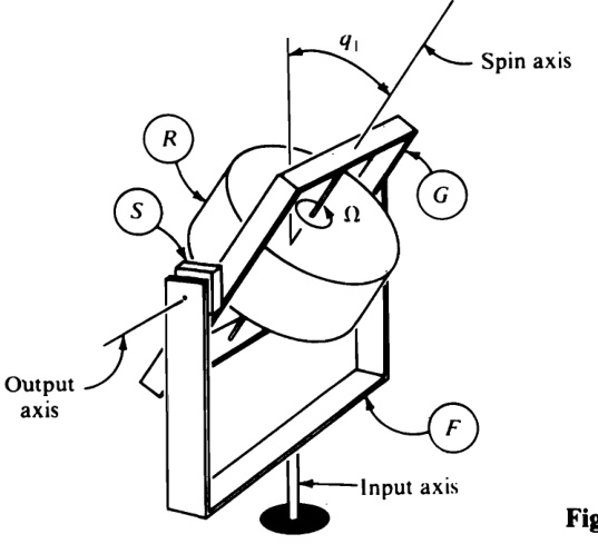
Figure P13.8

Result \frac{(4J\Omega/\pi)^{2}}{3(A+C+I+J+2D)}

13.9 Referring to the example in Sec. 7.4, suppose that the set of friction forces exerted on \boldsymbol{s} by T is treated as equivalent to a couple of torque -c\pmb{u}_{1}\pmb{e}_{1} (see Fig. 7.4.1), where ^c is a positive constant. Taking u_{1}=u_{4}=\dot{0} and u_{5}=4c(R-r)/(m r^{2}) at t=0 , show that \pmb{u_{4}} approaches a limiting value {{u}_{4}}^{*} as \boldsymbol{t} approaches infinity, and plot {u_{4}}/{u_{4}}^{*} versus c t/(m r^{2})

Result Figure P13.9

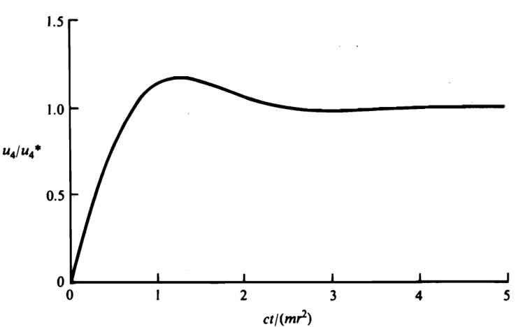
Figure P13.9

13.10 Considering the system s introduced in Problem 12.3, and letting u_{r}\triangleq{\dot{q}}, ， (r=1,2) (a) formulate exact dynamical equations of s.\left(b\right) Taking m_{A}= {\bf0.01\ k g,} m_{B}=0.1\;\mathbf{kg} L_{A}=0.075\;\mathrm{m} L_{B}=0.2\;\mathrm{m} A_{1}=5.0\,\times\,10^{-\,6}\,\mathrm{kg}\;\mathrm{m}^{2} B_{1}= 2.5\,\times\,10^{-4}\,\mathbf{kg}\,\mathbf{m}^{2} B_{2}=5.0\,\times\,10^{-\,5}\,\mathrm{kg\,m}^{2} , and B_{3}=2.0\,\times\,10^{-4}\,\mathrm{kg\,m}^{2} , perform a numerical simulation of the motion of s for 0\leq t\leq10\,{\mathrm{s}}, using for initial conditions u_{1}(0)=u_{2}(0)=0, q_{1}(0)=45^{\circ}, q_{2}(0)=1^{\circ} , and plot q_{2} versus t. Leaving all other quantities unchanged, but taking q_{2}(0)=0.5^{\circ} , make another plot of q_{2} versus t, and display the two curves on the same set of axes. (c) Repeat part (b) with q_{1}(0)=90^{\circ}

Compare the set of two curves generated in part (b) with the set obtained in part (c)_{\cdot} , and briefly state your conclusions.

Results

\begin{array}{r l}&{(a)\,\dot{u}_{1}=[2u_{1}u_{2}s_{2}\,\mathsf c_{2}(B_{1}-B_{2})-(m_{A}L_{A}+m_{B}L_{B})\mathsf g s_{1}]/(A_{1}+B_{1}\mathsf c_{2}^{\,2}+B_{2}\mathsf s_{2}),}\\ &{\qquad\qquad+\,m_{A}L_{A}^{\,2}+m_{B}L_{B}^{\,2});}\\ &{\qquad\dot{u}_{2}=-{u_{1}}^{2}s_{2}\mathsf c_{2}(B_{1}-B_{2})/B_{3}}\end{array} 22
(b) Fig. P13.10(a)
(c) Fig.P13.10(b)

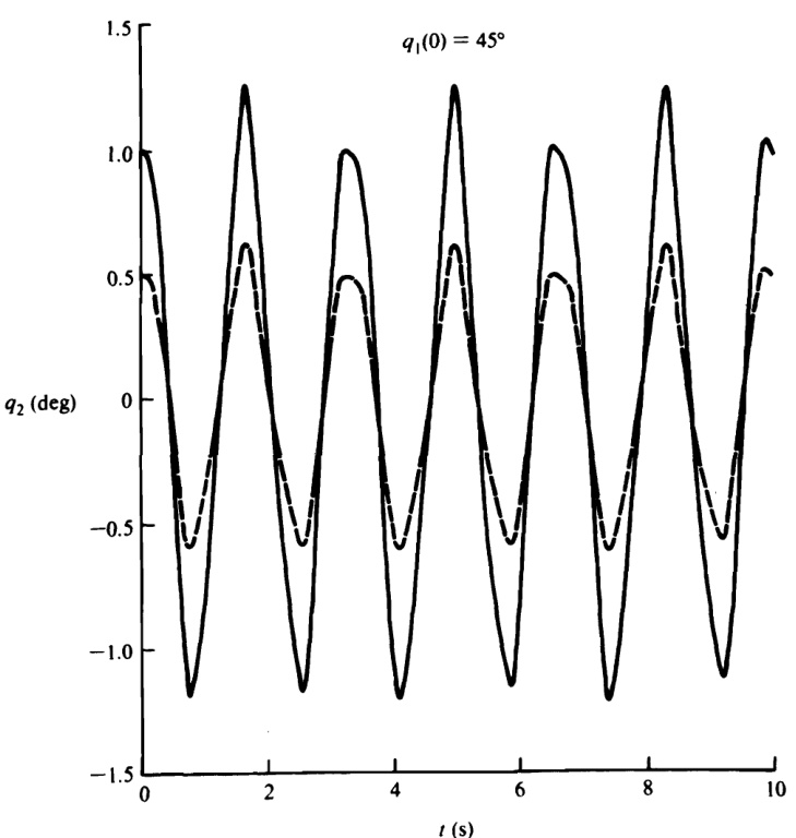
Figure P13.10(a)

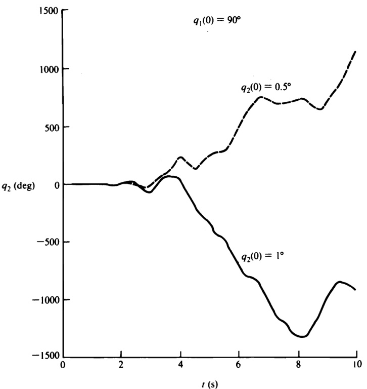
Figure P13.10(b)

*_{13.11} Referring to Problem 3.15 (see also Problems 4.17, 8.14, 8.20, 8.21, 10.10, 11.7, 11.8, and 13.5), take L_{A}=0.3\,\textrm{m} L_{B}=0.5\,\mathrm{~m~} L_{p}=1.1\,\mathrm{~m~} p_{1}=0.2\,\textrm{m} ， p_{2}=0.4\,\mathrm{m},p_{3}=0.6\,\mathrm{m},A_{1}=11\,\mathrm{kg}\,\mathrm{m}^{2},B_{1}=7\,\mathrm{kg}\,\mathrm{m}^{2},B_{2}=6\,\mathrm{kg}\,\mathrm{m}^{2},B_{3}=2 B_{3}=2\,\mathbf{k}\mathrm{g}\,\mathbf{m}^{2} C_{1}=5\;\mathbf{kg}\;\mathbf{m}^{2} ， C_{2}=4\mathrm{~kg~m}^{2} ， C_{3}=1\mathrm{~kg~m}^{2} ， D_{11}=2~\mathbf{kg}~\mathbf{m}^{2} ， D_{22}=2.5\;\mathrm{kg}\;\mathrm{m}^{2} ， D_{33}=1.3\;{\bf k g}\;{\bf m}^{2} ， D_{12}=0.6\;\mathbf{kg}\;\mathbf{m}^{2} ， D_{23}=0.75\;\mathrm{kg}\;\mathrm{m}^{2} ， D_{31}=\mathrm{~-~}1.1~\mathbf{kg}~\mathbf{m}^{2} m_{A}= \mathbf{87\,kg} m_{B}=63\,{\bf k g}, m_{c}=42\,{\bf k g}, $m_{D}=50,{\bf k g.},($ (a) Setting u_{1}(0)=0.1\;\mathrm{rad/s}, u_{2}(0)= \left[0\right)=0.3\,\mathrm{m}/\mathrm{s},q_{1}(0)=30^{\circ},q_{2}(0)=0.1\,\mathrm{m},q_{3}(0)=10^{\circ},T_{1}^{E/A}=T_{2}^{\ A/B}= K_{3}^{~\,B/C}=0, determine the value of K+V_{\mathrm{v}} (see Problem 10.10) at t=0 and t=5\,{\mathsf s} ， and the value of \mathbf{H}\cdot\mathbf{a}_{1} (see Problem 13.5) at t=0 and t=5\,{\mathbf s};(b) setting T_{2}{}^{A/B}= 10\:\mathrm{\bfN}\;\mathrm{\bfm} and \begin{array}{r}{K_{3}^{\phantom{},B/C}=20\,\mathrm{N},}\end{array} but leaving all other quantities as in (a) , determine the value of K+V_{v} at t=0 and t=5\,{\mathsf{s}} , and the value of \mathbf{H}\cdot\mathbf{a}_{1} at t=0 and t=5\,{\mathsf{s}} (c) the robot arm can be brought from an initial state of rest in E to a final state of rest in {\pmb E} such that q_{1},\,q_{2} , and \pmb q_{3} have the specified values q_{1}^{\mathrm{~*~}},q_{2}^{\mathrm{~\*~}} , and {q_{3}}^{*} ， respectively, by using the following feedback control laws:

\begin{array}{l}{{T_{1}^{E/A}=\,-\beta^{E/A}u_{1}\,-\gamma^{E/A}(q_{3}\,-\,q_{3}\,^{*})\qquad\qquad\qquad\quad\cdot}}\\ {{T_{2}^{A/B}=\,-\beta^{A/B}u_{2}\,-\,\gamma^{A/B}(q_{1}\,-\,q_{1}\,^{*})+\,g[(m_{B}L_{B}\,+\,m_{C}Z_{9}\,+\,m_{D}Z_{14})c_{1}\,-\,m_{D}p}}\\ {{K_{3}^{B/C}=\,-\beta^{B/C}u_{3}\,-\,\gamma^{B/C}(q_{2}\,-\,q_{2}\,^{*})+\,g(m_{C}\,+\,m_{D})s_{1}\,\qquad\qquad\qquad\quad\,}}\end{array}
$$\`S]  

![](images/fcbf7aac6924953f01ba3897bd676babfbae320e1a2c15f31c6e746bd899e758.jpg)  

Figure P13.11(a)  

![](images/e80464755887cfa82ba46d5fc0b72305c41d5a30e8c55fa8f210a2ea72c4b35e.jpg)  

Figure P13.11(b)  

![](images/ccba1ff7d4ae4943cd5c17066392362282e4c851546e661b67e6053dcdca4678.jpg)  
Figure P13.11(c)  

Here, $\beta^{E/A},\,\gamma^{E/A},\,\beta^{A/B},\,\gamma^{A/B},\,\beta^{B/C},$ and $\gamma^{B/C}$ are constant “ gains,” and the terms involving $\pmb{g}$ in the expressionsfor $T_{2}^{\,A/B}$ and $K_{3}^{\,\,\,B/C}$ serveto counteract the effects of gravity. Using these control laws, the parameter values employed previously, and $u_{1}(0)=u_{2}(0)=u_{3}(0)=0,q_{1}(0)=30^{\circ},q_{2}(0)=0.1\,\mathrm{m},q_{3}(0)=10^{\circ},q_{1}^{\circ}=$ ${q_{1}}^{*}=60^{\circ}.$ $q_{2}{}^{*}=0.4\mathrm{~m~}$ ， $q_{3}{}^{*}=70^{\circ}$ $\beta^{E/A}=464\mathrm{~N~m~s};$ $\gamma^{E/A}=306\mathrm{~N~m~}$ $\beta^{A/B}=216\mathrm{~N~m~s},$ $\gamma^{A/B}=285\mathrm{~N~m~}$ ， $\beta^{B/C}=169\,\mathrm{~N~s~}$ $\gamma^{B/C}=56~\mathrm{N},$ plot the values of $q_{1},\,q_{2}$ , and $\pmb q_{3}$ from $t=0$ to $t=15\:\mathbf{s}$  

# Results  

13.12 Referring to the example in Sec. 7.6, replace the set of forces exerted on the left half of $^{c}$ by the right half with a couple together with a force $\sigma_{1}\mathbf{n}_{1}+\sigma_{2}\mathbf{n}_{2}$ ， applying this force at the right end of the left half of $c$ For the values of $m_{A},m_{B}$ ， $m_{C},L,q_{1}(0),$ and ${\pmb u}_{1}(0)$ used in the example in Sec. 7.6, show that $\sigma_{1}=-(g/16)$ tan $\pmb{q}_{1}$ ， anddetermine $\pmb{\sigma_{1}}$ for $t=5\:{\mathsf s}$  

![](images/dc6bab4027094438c54ea2249cd53865022fc6d6b7a0764d86aea99afa5aca47.jpg)  
Figure P13.12  

Suggestions: Regard $c$ as composed of two identical bars, $C_{1}$ and $C_{2}$ , each of length $L$ and mass $m_{c}/2$ which can slide relative to each other as indicated in Fig. P13.12, and let $\boldsymbol{P}_{1}$ and $\boldsymbol{P}_{2}$ be the points of $C_{1}$ and $C_{2}$ , respectively, corresponding to the midpoint of $c$ .Note that during the motion of interest the velocity of $P_{2}$ in $C_{1}$ and the angular velocities of $C_{1}$ and $C_{2}$ can be expressed as  

{\bf c}{1}{\bf v}^{P{2}}=v{\bf n}{1}\qquad{\bf0}^{C{1}}={\bf0}^{C_{2}}=\gamma{\bf n}_{3}

  

where $\pmb{v}$ and $\gamma$ are functions of $\boldsymbol{q}_{1}$ and $\pmb{u}_{1}$ . Introduce $\pmb{u}_{2}$ as $u_{2}\triangleq\pmb{\omega}^{B}\cdot\pmb{\Pi}_{3}$ , and verify that the velocities of $\boldsymbol{P}_{1}$ and $\scriptstyle P_{2}$ are given by  

\mathbf{v}^{P_{1}}=2L u_{1}\mathbf{e}{1}+L(u{2}-u_{1})s_{1}\mathbf{n}_{2}

  

and  

\mathbf{v}^{P_{2}}=2L u_{2},\mathbf{e}{1}-L(u{2},-,u_{1})\mathbf{s}{1}\mathbf{n}{2}

  

Result $\sigma_{1}\,=\,-0.173\;\mathrm{N}$  

13.13 The system described in Problem 8.7 is at rest with $q_{1}=q_{2}=q_{3}=45^{\circ}$ Letting $\textbf{\emph{B}}$ designate the third bar from the left in the middle row of bars (the row in which the bars make an angle $\boldsymbol{q}_{2}$ with the vertical), determine the magnitude of the reaction of $\pmb{B}$ on the pin supporting the upper end of $\pmb{B}$  

Suggestion: Regard the upper end of $\pmb{B}$ as disconnected from the pin that supports this end, and note that the six bars shown in Fig. $\mathbb{P}13.13(a)$ aremovable  

344 PROBLEM SETS  

![](images/7fb6443d0ddb1711d5c469cfbc91081ea9c77fd577e660948e40d53b5e50ff2e.jpg)  
Figure P13.13  

under these circumstances, whereas the rest of the bars are not movable so long as $q_{1},\,q_{2}$ , and $\mathbf{q_{3}}$ have fixed values. Introduce generalized speeds $\pmb{u_{4}}$ and $\pmb{u_{5}}$ such that bars $\pmb{B}$ and $^{c}$ have counterclockwise angular velocities, as indicated in Fig. $\mathbb{P}13.13(a)$ .Record the velocities of the mass centers of the movable bars and the velocity of the upper end of $\pmb{B}$ as in Fig. $\mathbf{P}13.13(b).$ ,and use this sketch to depict partial velocities associated with u4 as in Fig. P13.13(c). Record the gravitational forces acting on the sixbars,as well as thehorizontal andvertical reactionforce components at theupper endof $\pmb{B}$ as in Fig. $\lceil13.13(d)$ .Refer to Figs. $\mathbb{P}13.13(c)$ and $\mathbf{P}13.13(d)$ to perform by inspection the dot-multiplications required to form the generalized active force $\pmb{F_{4}}$ , thus verifying that $F_{4}=L(-R_{2}+4m g)$ . Make a sketch similar to Fig. $\mathbf{P}13.13(c)$ to depict the partial velocities associated with $\pmb{u_{5}}$ ， and use this sketch in conjunction with Fig. P13.13(d) to form an expression for the generalized active force $\boldsymbol{F}_{5}$ . Finally, appeal to Eqs. (6.5.2) to find $\pmb{R}_{1}$ and $\pmb{R}_{2}$  

# Result 113mg/2  

$\bf{*13.14}$ Referring to the example in Sec. 6.6, verify that there exist values of $\pmb{\theta}$ $(0<\theta<\pi/2)$ : such that the steady motion there considered cannot occur. For  

$0\leq h/R\leq2;$ show that these values of $\theta$ correspond to the shaded region of Fig.   
P13.14.  

![](images/ce184f957f76c9950f2fa306ad6faeff1bcee651ff99084852ec038fa50d2ac3.jpg)  
Figure P13.14  

13.15Taking $L\Omega^{2}/g=3;$ determine two pairs of constant values of $\pmb q_{1}$ and $\pmb q_{2}$ such that the equations of motion of the system considered in the example in Sec. 6.7 are satisfied, and sketch the system in the configuration associated with each pairofvalues.  

Results $q_{1}=56.18^{\circ};$ $q_{2}=226.30^{\circ}$ $q_{1}=74.25^{\circ}$ ， $q_{2}=78.34^{\circ}$ ; Fig. P13.15  

![](images/f90ffed74e593625325b45664e857e830e1b70ac052c7cf8236c6b937dc6d2d6.jpg)  
Figure P13.15  

# PROBLEM SET 14  

(Secs. 7.8-7.10)  

14.1 A rigid body $\textbf{\emph{B}}$ forms part of a simple nonholonomic system $s$ possessing $n\mathrm{~-~}m$ degrees of freedom in a Newtonian reference frame $N$ . Letting $\mathbf{L}$ and $\mathbf{H}$ denote, respectively, the linear momentum of $\pmb{B}$ in $N$ and the central angular momentum of $\textbf{\emph{B}}$ in $N$ , show that the contribution of $\textbf{\emph{B}}$ to the generalized momenta $p_{1},\ldots,p_{n-m}$ can be expressed as  

(p_{r}){B}=\tilde{\pmb{\upsigma}}{r}\cdot{\bf H}+\tilde{\bf{v}}_{r}^{;*}\cdot{\bf L};;;;;;;(r=1,\ldots,n-m)

  

where $\tilde{\mathbf{o}}_{r}$ and $\tilde{\mathbf{v}}_{r}^{\ast}$ are, respectively, the rth nonholonomic partial angular velocity of $\pmb{B}$ in $N$ and the rth nonholonomic partial velocity of the mass center of $\pmb{B}$ in $N$  

14.2 A rigid body $\pmb{B}$ is a part of a simple nonholonomic system ${\boldsymbol s}$ possessing $n\mathrm{~-~}m$ degrees of freedom in a Newtonian referenceframe $N$ andasubset $\pmb{\sigma}$ of the contact forces acting on particles of S consists of forces applied to $\textbf{\emph{B}}$ and forming a couple oftorque T. Show that $(I_{r})_{\sigma}$ ,the contribution of the forces of $\pmb{\sigma}$ to the generalized impulse $I_{r}$ , is given by  

(I_{r}){\sigma}=\tilde{\otimes}{r}{}^{B}(t_{1})\cdot\int_{t_{1}}^{t_{2}}\mathbf{T};d t;;;;;;;(r=1,\ldots,n-m)

  

where $\tilde{\omega}_{r}{}^{B}(t_{1})$ is the value at time $t_{1}$ of the rth nonholonomic partial angular velocity of $\pmb{B}$ in $N$ , and $t_{2}$ differs so little from $t_{1}$ that the configuration of $s$ in $N$ does not change significantly during the time interval beginning at $t_{1}$ and endingat $t_{2}$  

14.3 Referring to Problem 4.11, let $P$ be a horizontal plane, and let $\pmb{A}$ be a Newtonian reference frame. Show that when $C_{1}$ and $C_{2}$ roll on $P$ $s^{*}$ moves on a circle, and determine the radius of the circle when the system is set into motion by a blow applied to $s$ along a line that intersects the axis of $\boldsymbol{s}$ at a distance s from $s^{*}$ .Assume that no slipping occurs, and express the result in terms of the radius $\pmb R$ and length $L$ shown in Fig. P4.11, as well as the mass $m_{s}$ of $\pmb{S}$ , the mass $m_{c}$ of each of $C_{1}$ and $C_{2}$ , the central transverse moment of inertia $J$ of $\pmb{S}$ , and the axial moment of inertia $\boldsymbol{\mathit{I}}$ of each of $C_{1}$ and $C_{2}$ , letting $C_{1}$ and $C_{2}$ each have a transverse central moment of inertia $I/2$  

Result $\frac{I+J+2(m_{C}+I/R^{2})L^{2}}{s[m_{S}+2(m_{C}+I/R^{2})]}$  

14.4 Four identical uniform rods, each of length $_{2L}$ areconnectedby smooth pins so as to form a square, and are resting on a smooth, horizontal surface when one of the rods is struck,the line of action of the biowpassing through one corner of the square, as shown in Fig. P14.4. Determine the distance $h$ suchthatthesystem moves as if it were a rigid body subsequent to being struck.  

![](images/ec6fd7d19847f79ff0695de152d2b30b81cc70d04c9c998284b866507309f5dc.jpg)  
Figure P14.4  

Result $h=4L/3$  

14.5 In Fig. P14.5, $\mathbf{n}_{1}$ $\mathbf{n}_{2}$ , and $\mathbf{n}_{3}$ are mutually perpendicular unit vectors fixed relative to a horizontal plane $H$ in such a way that $\mathbf{n}_{2}$ isperpendicular to $\boldsymbol{H}$ $\boldsymbol{S}$ is a thin,uniform spherical shell that,at a certain instant,strikes $H$ at a point $A$ of $H$ the velocity $\mathbf{v}^{*}$ of the center of $s$ and the angular velocity $\mathbf{\boldsymbol{\Theta}}$ of $s$ at this instant being given by  

\begin{array}{r l r}&{\mathbf{v}^{*}=10(-\mathbf{n}{2}+\mathbf{n}{3})\quad\mathrm{~m/s}}&\ &{\mathbf{o}=100(\mathbf{n}{1}+2\mathbf{n}{2}+5\mathbf{n}_{3})\quad\mathrm{~rad/s}}\end{array}

  

Thereafter, $s$ bounces from $A$ to $B_{\cdot}$ from $B$ to $C$ and so forth.  

![](images/963e3a034a91d45a1b667a5d89a9fab35cc80abdc1cb8c9f6099e69a7bbbdd04.jpg)  
FigureP14.5  

Letting the coefficient of restitution for $S$ and $H$ have the value 0.5, taking the coefficients of static friction and kinetic friction equal to 0.25 and 0.20, respectively, and setting $b=0.03\textrm{m}$ determine the distance from $A$ to $C$  

Result 13.90m  

14.6 In Fig. $\mathbf{P}14.6(a)$ $\pmb{A}$ and $\pmb{B}$ are uniform rods, each having a length of $_{2\textrm{m}}$ and a mass of $3\;\mathbf{kg}.$ . The two rods form a double pendulum moving in such a way that, at a certain instant, the free end of $\textbf{\emph{B}}$ strikes a horizontal surface $H$ while the angular velocities of $\pmb{A}$ and $\pmb{B}$ have magnitudes of 0.1 rad/s and $0.2\;\mathrm{\bfrad/s}$ ,respectively, and are directed as shown.  

$(a)$ If $e$ , the coefficient of restitution for $\pmb{B}$ and $H$ , has the value 0.5, what is the minimum value that $\pmb{\mu}$ , the coefficient of static friction for $\pmb{B}$ and $\pmb{H}$ , must have in order for $\pmb{B}$ not to be sliding on $H$ at the instant of separation ?  

$(b)$ If $e=0.5$ $\mu=0.25$ , and $\mu^{\prime}=0.20$ ,where $\mu^{\prime}$ is the coefficient of kinetic friction for $\pmb{B}$ and $H$ , what are the angular velocities of $\pmb{A}$ and $\pmb{B}$ immediately after impact? Draw a sketch of the system, showing the angular velocities of $\pmb{A}$ and $\pmb{B}$  

(c) For each of the sets of values of $e,\,\pmb{\mu},$ and $\mu^{\prime}$ in Table $\mathbb{P}14.6(a)$ determine whether or not slipping is taking place at the instant of separation, whether the kinetic energy increases or decreases during the collision, and the amount of kinetic energychange.  

Results (a) 0.431 (b) Fig. $\mathbf{P}14.6(b)$ (c) Table P14.6(b)  

![](images/c5b44590ad038de12fc15880d0b041e0d6114436928a38db119e585d77f65914.jpg)  
Figure P14.6(a)  

![](images/13708835728dc93b3651eac6a0374d06ce8e0a81b4fa8cd30da9a53aa7d4af85.jpg)  
Figure P14.6(b)  

Table P14.6(a)   


<html><body><table><tr><td>e</td><td>μ</td><td>μ'</td></tr><tr><td>0.5</td><td>0.25</td><td>0.20</td></tr><tr><td>0.5</td><td>0.50</td><td>0.40</td></tr><tr><td>0.3</td><td>0.50</td><td>0.40</td></tr><tr><td>0.7</td><td>0.51</td><td>0.50</td></tr></table></body></html>  

Table P14.6(b)   


<html><body><table><tr><td>e</td><td>μ</td><td>u'</td><td>Slipping</td><td>Kinetic energy change</td></tr><tr><td>0.5</td><td>0.25</td><td>0.20</td><td>Yes</td><td>0.03N m decrease</td></tr><tr><td>0.5</td><td>0.50</td><td>0.40</td><td>No</td><td>0.16 N m increase</td></tr><tr><td>0.3</td><td>0.50</td><td>0.40</td><td>No</td><td>0.12 N m decrease</td></tr><tr><td>0.7</td><td>0.51</td><td>0.50</td><td>Yes</td><td>0.49 N m increase</td></tr></table></body></html>  

14.7 A system moving in accordance with Eq. (7.10.1) is said to be performing undampedfreevibrationsif  

n=f(t)=0

  

Making use of Euler's identities  

e^{\pm,i q}=\cos{,q}\pm,i\sin{,q}

  

where $i$ is the imaginary unit and $q$ is any real quantity, verify that under these circumstances $_{x}$ can be expressed as  

x=x(0)\cos p t+{\frac{\dot{x}(0)}{p}}\sin p t

  

Showthat $T,$ . called the period of the motion and defined as the shortest time between two instants at which $_{x}$ attains stationary values (values such that $\dot{\boldsymbol{x}}=\boldsymbol{0}$ of the same sign, is given by  

T={\frac{2\pi}{p}}

  

Taking ${\dot{\mathbf{x}}}(0)=0$ plot $x/x(0)$ versus pt for $0\le p t\le20$  

Result Figure P14.7  

![](images/07f950c165656e376fcad94be7b0465f8f59d232368b08d926f13c07b48ffddf.jpg)  

# Figure P14.7  

14.8 A system moving in accordance with Eq. (7.10.1) is said to be performing underdampedfreevibrationsif  

0<n<1\qquad f(t)=0

  

# 350 PROBLEM SETS  

Show that during such vibrations  

x=\Big{x(0)\cos[p(1-n^{2})^{1/2}t]+\frac{\dot{x}(0)+n p x(0)}{p(1-n^{2})^{1/2}}\sin[p(1-n^{2})^{1/2}t]\Big}e^{-n p t}

  

and verify that the period $T,$ . defined as in Problem 14.7, is given by  

T=\frac{2\pi}{p(1-n^{2})^{1/2}}

  

![](images/df8738596f088b08023bcee9fea82e4a7e6cd56389c970326e61225402e32589.jpg)  

Figure P14.8(a)  

![](images/bfd2bf42bd6b368f743c0a6d885a52e76532bfa8dae6515cf4560240c0ee9b2a.jpg)  

Figure P14.8(b)  

Showthat $\delta$ , the logarithmic decrement, defined as the natural logarithm of theratio of ${\boldsymbol{x}}(t)$ to $x(t+T),$ , can be expressed as  

\delta=n p T

  

Taking $\dot{\mathfrak{x}}(0)=0$ and $n=0.2,$ plot $\mathbf{\boldsymbol{x}}/\mathbf{\boldsymbol{x}}(0)$ versus pt for $0\le p t\le20.$ Repeat with $n=0.1$  

Results Figures P14.8(a), P14.8(b)  

14.9 A system moving in accordance with Eq. (7.10.1) is said to be performing critically damped free vibrations if  

\begin{array}{r}{n=1\qquad f(t)=0}\end{array}

  

Referring to Problem 14.8, use a limiting process to verify that  

x={[\dot{x}(0)+p x(0)]t+x(0)}e^{-p t}

  

and show that there exists at most one value of $t$ such that $_{x}$ has a stationary value. Taking $x(0)=0$ plot $\boldsymbol{x}/\boldsymbol{x}(0)$ versus pt for $0\le p t\le20.$  

Result Figure P14.9  

![](images/477b6deeb53f817690a10f4edb60d4fb819b80b0d43a2b497851d40ef4ad6498.jpg)  

Figure P14.9  

14.10 A system moving in accordance with Eq. (7.10.1) is said to be performing overdampedfreevibrationsif  

n>0\qquad f(t)=0

  

After verifying that $_{x}$ is given by  

x=\frac{1}{a_{1},-a_{2}},{[\dot{x}(0),-,a_{2},x(0)]e^{a_{1}t},-,[\dot{x}(0),-,a_{1}x(0)]e^{a_{2}t}}

  

where $\pmb{a}_{1}$ and $\pmb{a}_{2}$ are real quantities given by Eqs. (7.10.3), show that, once again (see Problem 14.9), there exists at most one value of $t$ suchthat $_x$ has a stationary value.  

Taking $\dot{\boldsymbol{x}}(0)=0$ and $n=3$ plot $x/x(0)$ versusptfor $0\le p t\le20.$  

Result Figure P14.10  

![](images/e59ad99a67f595259120fc961e2e2716fd95284ea110b5918fa32c10d4ba5567.jpg)  

Figure P14.10  

14.11 A system moving in accordance with Eq. (7.10.1) is said to be performing dampedharmonicallyforcedvibrationsif  

n>0\qquad f(t)=b,\sin(\omega t+\phi)

  

where $b,\,\omega,$ and $\phi$ are constants called, respectively, the amplitude, the circular frequency, and the phase angle of the forcing function.  

Show that $x$ can be written as  

\boldsymbol{x}=\boldsymbol{x}{s}+\boldsymbol{x}{T}

  

where $\pmb{x_{s}}$ and $x_{T}$ , respectively called’ the steady-state response and the transient response, aregiven by  

x_{s}={\frac{b(\beta_{1},\sin,\omega t,+,\beta_{2},\cos,\omega t)}{(p^{2},-,\omega^{2})^{2},+,(2n p\omega)^{2}}}

  

and  

x_{T}=\frac{\alpha_{1}e^{a_{1}t}-\alpha_{2}e^{a_{2}t}}{2p(n^{2}-1)^{1/2}}

  

with $\pmb{\alpha}_{i}$ and $\beta_{i}\,(i=1,2)$ defined as  

\begin{array}{r l}&{\alpha_{1}\triangleq\dot{x}(0)-a_{2}x(0)+\frac{b}{a_{1}^{2}+\omega^{2}}\left(a_{1}\sin\phi+\omega\cos\phi\right)}\ &{\alpha_{2}\triangleq\dot{x}(0)-a_{1}x(0)+\frac{b}{a_{2}^{2}+\omega^{2}}(a_{2}\sin\phi+\omega\cos\phi)}\ &{\beta_{1}\triangleq2n p\omega\sin\phi+(p^{2}-\omega^{2})\cos\phi}\ &{\beta_{2}\triangleq(p^{2}-\omega^{2})\sin\phi-2n p\omega\cos\phi}\end{array}

  

![](images/97b2c6e39b0ee28c5ceb7bcb28a350774ec5663cd3059c148b5500708beab6a1.jpg)  

Figure P14.11(a)  

![](images/278deb12434166acad11058992937cd816c3aa6af52004daf027e5a0319ad90d.jpg)  

Figure P14.11(b)  

and $a_{i}\,(i=1,2)$ given by Eqs. (7.10.3). Verify that  

\operatorname*{lim}{t\to\infty},x{T}=0

  

and that the absolute value of the maximum value of $x_{s}$ , called the steady-state amplitude,isgivenby  

|(x_{S})_{\mathrm{max}}|=|b|[(p^{2}-\omega^{2})^{2}+(2n p\omega)^{2}]^{-1/2}

  

Taking $\dot{x}(0)=0,\,n=0.3,\,b=x(0)p^{2},\,\phi=0,$ and $\omega=2p$ ,plot $x/x(0)$ versus pt for $0\le p t\le20.$ Repeat with $\omega=p$  

Results Figures P14.11(a), P14.11(b)  

14.12 A system moving in accordance with Eq. (7.10.1) is said to be performing undampedharmonicallyforcedvibrationsif  

n=0\qquad f(t)=b,\sin(\omega t+\phi)

  

where $b,\omega_{:}$ and $\phi$ are constants (see Problem 14.11).  

After verifying that, so long as $\omega$ differs from $p,x$ is given by  

\begin{array}{l}{{x=x(0)\cos,p t+\displaystyle\frac{\dot{x}(0)}{p}\sin,p t+\frac{b}{p^{2}-\omega^{2}}\left[\left(\sin,\omega t-\frac{\omega}{p}\sin,p t\right)\cos,\phi\right.}}\ {{\left.\qquad+\left(\cos,\omega t-\cos,p t\right)\sin,\phi\right]\qquad}}\end{array}

  

show by means of a limiting process that resonance, that is, the response obtained when $\omega=p$ ischaracterizedby  

x=x(0)\cos{p t}+\left[{\frac{\dot{x}(0)}{p}}+{\frac{b\cos{\phi}}{2p^{2}}}\right]\sin{p t}-{\frac{b t}{2p}}\cos(p t+\phi)

  

Taking $\dot{x}(0)=0,b=x(0)p^{2},\omega=p$ and $\phi=0$ plot $\mathbf{\boldsymbol{x}}/\mathbf{\boldsymbol{x}}(0)$ versus pt for $0\leq p t\leq$ 150.  

When the behavior of a system is characterized by a curve such as the one in Fig. $\mathbf{P}14.12(b),$ . beats are said to be taking place. Show that setting ${\dot{\mathbf{x}}}(0)=0,$ $\phi=\pi/2$ and $b=x(0)p^{2}$ leadsto  

x=x(0)\cos{p t}-\frac{2x(0)}{1-\omega^{2}/p^{2}}\sin\biggl[\biggl(\frac{p+\omega}{2}\biggr)t\biggr]\sin\biggl[\biggl(\frac{p-\omega}{2}\biggr)t\biggr]

  

Taking $\omega=0.9$ plot $x/x(0)$ versuspt for $0\leq p t\leq150$ to verify that the above equation describes beats under these circumstances.  

Results Figures P14.12(a), P14.12(b)  

![](images/ed927e3c9d3bf9bbb9b20a2fbbec296c575c157069c52b4988328831bc9220dd.jpg)  
Figure P14.12(a)  

![](images/c32e3eea626f2570e815cf89512f9a321bb04bd68fbdef9c97dd4577340a3aa1.jpg)  
Figure P14.12(b)  

14.13 A variable-speed motor is supported by a horizontal floor. When in operation, it performs vertical vibrations giving rise to the following observations.  

When the rotor is turning at a constant angular speed, the amplitude of the vertical displacement of the motor casing from the casing's rest position is greatest if the angular speed is equal to $1000\ \mathrm{rpm}$ ; the greatest amplitude has a value of $0.011\textbf{m}$ Once the motor has been turned off so that the rotor remains at rest relative to the stator, vibrations with decaying amplitude take place with a frequencyof $16\:\mathbf{Hz}$  

Determine at what constant angular speeds below $3000\;\mathrm{rpm}$ the motor may not be operated if the amplitude of the vertical displacement is not to exceed $0.005\,\mathrm{m}$ For operation in the permitted range of angular speeds, find the maximum value of the ratio of $\pmb{F}$ to the weight of the motor, $\pmb{F}$ being the magnitude of the force transmitted to the floor by the motor casing.  

![](images/756b70a77b7b7731f7ab866ed64a0bd53fa05404167a640e7d78292c9bb72d43.jpg)  

Figure P14.13(a)  

![](images/6b0e9788b6a07c8cbe2c2267045e0a81df93c99ddb3aa8ee0c39595c4fd170de.jpg)  

Figure P14.13(b)  

Suggestion: Regard the motor as consisting of a rigid stator that carries a rotor whose mass center does not lie on the axis of rotation of the rotor, and let the motor be supported by a linear spring S and linear damper $\pmb{D}$ , as indicated in Fig. $\mathbb{P}14.13(a).$ where $G_{1}$ designates the mass center of the stator, $\pmb R$ is the distance from $\pmb{A}$ , the axis of rotation of the rotor, to $G_{2}$ , the mass center of the rotor. Let $\pmb{h}$ be the static displacement of $\pmb{A}$ from the position $\pmb{A}$ occupies when $\boldsymbol{s}$ is unstretched, and let $x$ be the displacement of $\pmb{A}$ from the static equilibrium position of $\pmb{A}$ to the position of $\pmb{A}$ at any time. Verify that $_x$ is governed by the equation  

\ddot{x}+2n p\dot{x}+p^{2}x=R\bigg(\frac{M^{\prime}}{M}\bigg),\omega^{2}\cos{\omega t}

  

where $M$ and $M^{\prime}$ are the masses of the entire motor and of the rotor, respectively, $\omega$ is the (constant) angular speed of the rotor, $p^{2}=g/h_{*}$ and $2n p=C/M,C$ being the damping constant associated with $\pmb{D}$ Plot thedisplacement amplificationfactor $\pmb{\alpha},$ defined as $\alpha\triangleq\lvert x_{\mathrm{max}}\rvert/h_{\mathrm{;}}$ . and the force amplification factor $\beta_{:}$ defined as $\beta$ = $F_{\mathrm{max}}/(M g)$ , as functions of $\omega/p$ for $0\leq\omega/p\leq3$ [see Fig. $\mathbb{P}14.13(b)]$  

Results $775<\omega<1731\;{\mathrm{rpm}};[F/(M g)]_{\mathrm{max}}=7.1$ \*14.14 Referring to Problem 3.15 (see also Problems 4.17, 8.14, 8.20, 8.21, 10.10, 11.7, 11.8, 13.5, and 13.11), $^{(a)}$ let $\pmb{I}$ denote the moment of inertia of $A,B,C,$ and $\pmb{D}$ with respect to the hub axis of $\pmb{A}$ , let $\pmb{J}$ be the moment of inertia of $B,C_{\mathrm{i}}$ and $\pmb{D}$ with respect to the joint axis at $\pmb{P}$ and take $M=m_{C}+m_{D}$ .Show that (see Problem 11.7) $I=-\ensuremath{X_{11}}$ ， $J=-X_{22}$ , and $M=-X_{33}.\,(b)$ For the parameter values and values of $q_{1}(0)$ $q_{2}(0)$ , and $\ensuremath{\boldsymbol{q}}_{3}(0)$ used in Problem 13.11, determine $I,J,$ and $\pmb{M}$ (c) Taking $T_{1}^{~\pmb{E}/A}$ as in Problem 13.11 with ${q_{3}}^{*}=0$ and permitting only $\pmb q_{3}$ to vary, show that the equation of motion governing $\pmb q_{3}$ , linearized in $\pmb q_{3}$ , can be written  

\ddot{x}+2n p\dot{x}+p^{2}x=0

  

where $\mathbf{x}=q_{3}$ ， $2n p=\beta^{E/A}/I,$ and $p^{2}=\gamma^{E/A}/I$ ; proceeding similarly in connection with $\pmb q_{1}$ and $\pmb q_{2}$ ,showthat this equation applies also when $x=q_{1},2n p=\beta^{A/B}/J,$ and $p^{2}=\gamma^{A/B}/J_{\mathrm{~\,~}}$ in the case of $\pmb q_{1}$ , and when $x=q_{2}$ ， $2n p=\beta^{B/C}/M,$ and $p^{2}=\gamma^{B/C}/M,$ in the case of $q_{2}.\left(d\right)$ Referring to Problem 14.8, show that  

n=\left[1+\left(\frac{2\pi}{\delta}\right)^{2}\right]^{-1/2}

  

and determine $\delta$ and $\pmb{n}$ such that $x(t\,+\,T)/x(t)=1/100.$ (e) Taking $T=10\textbf{s},$ determine $\beta^{E/A},\,\gamma^{E/A},\,\beta^{A/B},\,\gamma^{A/B},\,\beta^{B/C}$ and $\gamma^{B/C}$ , each to the nearest whole number. $(f)$ Using the parameters and initial conditions employed in part $(c)$ of Problem 13.11, but assigning to $\beta^{E/A},\,\gamma^{E/A},\,\beta^{A/B},\,\gamma^{A/B},\,\beta^{B/C}$ and $\gamma^{B/C}$ the values found in part $(e)$ of the present problem, plot the values of $q_{1},q_{2}$ , and $\pmb q_{3}$ from $\boldsymbol{t=0}$ to $t=15\,{\sf s}.$ $\mathbf{\Pi}(g)$ Recompute, to the nearest whole number, the values of $\beta^{A/B},\;\gamma^{A/B},$ and ${\beta^{B/C}}$ with $T=5$ s. Compare the values of $\mathrm{~}^{\uparrow}\,\beta^{E/A},\;\gamma^{E/A},\;\beta^{A/B},\;\gamma^{A/B},\;\beta^{\dot{B}/C}$ and $\gamma^{B/C}$ now in hand with their counterparts in part $(c)$ of Problem 13.11. Compare Figs. $\mathbf{P}13.11(a){\bf-}\mathbf{P}13.11(c)$ with Figs. $\mathbf{P}14.14(a)–\mathbf{P}14.14(c)$ . What do you conclude?  

358 PROBLEM SETS  

![](images/a035121901e97ff1965edb682896ab249e6c8df1f1d30938b032effde751db91.jpg)  

Figure P14.14(a)  

![](images/3739270387d471e0e06743a69895f875be9d7afd8cfb39d7c123cad6a412ca5a.jpg)  

Figure P14.14(b)  

![](images/9b221f249a0f417f470d61be7e121ec2965d292d8bd19cb98b42493153ce5d7d.jpg)  

Figure P14.14(c)  

Results $\left(b\right)I=503.61\mathrm{~kg~m}^{2}\qquad J=117.37\mathrm{~kg~m}^{2}\qquad M=92\mathrm{~kg~}$ (d) $\delta=4.60517\qquad n=0.591155$ (e) $\begin{array}{r l}&{\beta^{E/A}=464\mathrm{~N~m~s~}\quad\gamma^{E/A}=306\mathrm{~N~m~}\quad\beta^{A/B}=108\mathrm{~N~m~s~}}\\ &{\gamma^{A/B}=71\mathrm{~N~m~}\quad\beta^{B/C}=85\mathrm{~N~s~}\quad\gamma^{B/C}=56\mathrm{~N~}}\end{array}$ $(f)$ Figures P14.14(a), P14.14(b), P14.14(c) $(g)~\beta^{A/B}=216\textrm{N m s}\qquad\gamma^{A/B}=285\textrm{N m}\qquad\beta^{B/C}=169\textrm{N s}$  

14.15 When a force $\mu k L\sin(\varepsilon\omega t)\mathbf{n}_{1}$ is applied to the particle $\boldsymbol{P}_{1}$ of the system considered in the example in Sec. 7.10, the differential equations governing the motion of S are Eqs. (7.10.51), with $M$ and $\pmb{K}$ as given in Eqs. (7.10.59) and (7.10.61), respectively, and  

F=\mu k L[\sin(\varepsilon\omega t)\quad0\quad0\quad0\quad0\quad0\quad0\quad0\quad0\quad0\quad0\quad0\quad0]^{T}

  

Taking $q_{r}(0)={\dot{q}}_{r}(0)=0$ $(r=1,\ldots,12)$ ， $\pmb{\mu}=0.01$ , and $\pmb{\varepsilon}=0.1$ plot $q_{1}/L$ versus ot for $0\leq\omega t\leq60,$ using 1, 3, and 12 modes. Next, using 12 modes, plot $q_{1}/L$ versus wt for $0\leq\omega t\leq60$ with $\pmb{\mu}=0.01$ and $\varepsilon=0.2586$ Comment briefly on the difference between the two $q_{1}/L$ versus wt curves obtained with 12 modes for $\varepsilon=0.1$ and $\varepsilon=0.2586$  

Results Figures P14.15(a), P14.15(b)  

360 PROBLEM SETS  

![](images/7eaf07fad48b89bbee7ac30ea8b41b02d71f1fe4f896979d9d5516ca53c3dc32.jpg)  

Figure P14.15(a)  

![](images/2aabf4274cb6fa73b7604c0f8c10a02781b4083d0470bfe62881ad443c60f725.jpg)  

# INERTIA PROPERTIES OF UNIFORM BODIES  

The information presented in Figs. A1-A28 applies variously to bodies modeled as matter distributed uniformly along a. curve, over a surface, or throughout a solid. In each case, the mass center of the body under consideration is identified by the letter $^{c}$ , and the length of the curve (Figs. A1-A4), area of the surface (Figs. A5-A20), or volume of the solid (Figs. A21-A28) used to model the body is recorded. To distinguish figures dealing with surfaces from those involving curves Or solids, shading is employed in Figs. A5-A20. For example, Figs. A18 and A24 apply to a spherical shell and a solid sphere, respectively.  

The symbols $I_{1},\,I_{2}$ , and $I_{12}$ in Figs. A1-A28 are defined as $I_{j}\triangleq\mathbf{n}_{j}\!\cdot\!\mathbf{I}\!\cdot\!\mathbf{n}_{j}$ $(j=1,2)$ and $I_{12}\triangleq\mathbf{n}_{1}\cdot\mathbf{I}\cdot\mathbf{n}_{2}$ , where I is the central inertia dyadic (see Sec. 3.6) of the body under consideration and $\mathbb{n}_{1}$ and $\displaystyle\mathbf{u}_{2}$ are orthogonal unit vectors shown in the figures. These unit vectors are parallel to central principal axes (see Sec. 3.8), except in the cases for which a product of inertia is reported (Figs. A5, A6, A12, A13, A17). A unit vector $\pmb{\mathbb{n}_{3}}$ , defined as $\mathbf{n}_{3}\triangleq\mathbf{n}_{1}\times\mathbf{n}_{2}$ is parallel to a central principal axis in all cases; and $I_{3}$ , the associated central principal moment of inertia, is given by $I_{3}=I_{1}+I_{2}$ for the bodies in Figs. A1-A17, but not for those in Figs. A18-A28. In connection with Figs. A18-A25, $I_{3}$ is equal to $I_{1}$ ; to obtain $I_{3}$ for the bodies in Figs. A26-A28, replace $^{c}$ with $\pmb{a}$ in the expression for $I_{1}$ .Finally, the symbol $m$ denotes in every case the mass of the body under consideration.  

# 362 INERTIA PROPERTIES OF UNIFORM BODIES  

![](images/963e991a0e1b1bf1bd69c1f273ea2567e8bb4b611a192b007530c9853d119240.jpg)  

\begin{array}{r}{I_{2}=\frac{m L^{2}}{12}}\end{array}

  

Figure A1  

![](images/d921aa2cfc9a2effb26cba651d446dc8e533639aabfb700ed3e751f8150153c8.jpg)  
Figure A2  

![](images/e1047b3b2c784cfd47a4ffafba558760005bf0f5e8deaf19f492a09a4f13f6f0.jpg)  

![](images/8228956711cfcb20df650dc1ad4e6b9abdc8e8f73657239cfe778bf38c200a20.jpg)  

$\begin{array}{l}{{I_{1}=\,\frac{m}{18}\Big(\frac{b\sin\theta}{a+c}\Big)^{\!\!2}(a^{2}+4a c+c^{2})}}\\ {{\ }}\\ {{I_{2}=\,\frac{m}{18(a+c)^{2}}\,\,[b^{2}(a^{2}+4a c+c^{2})\cos^{2}\theta}}\\ {{\ }}\\ {{\qquad\qquad\qquad+b(a^{3}+3a^{2}c-3a c^{2}-c^{3})\cos\theta}}\\ {{\ }}\\ {{\qquad\qquad\qquad+a^{4}+2a^{3}c+2a c^{3}+c^{4}]}}\end{array}$ $I_{12}=-\,\frac{m b\,\sin\theta}{36(a+c)^{2}}\,\,(a^{2}+4a c+c^{2})(2b\,\cos\theta+c-a)$  

![](images/9f749d10a691f48a0deeb6cbeb4be5b961c9ae86d6b998cc9bf362de08a25b78.jpg)  
Paralllogram  

Figure A5  

364INERTIA PROPERTIESOFUNIFORMBODIES  

![](images/b95284c8cdf518499cc87b3bbe6ace7c72c37cc7a906a8d186166058edfefbee.jpg)  
Figure A7  

![](images/b6b6527776c3a23496d4a6103a3ae85d4c9f572516b47658dee89eb21446f6a8.jpg)  
Area:OR2  

![](images/19cec15d533fdaee9c1effe3c1b6282e77572e9c25e87b4852b4eb1b54536f6d.jpg)  

![](images/072e5a2e25f80c18c78d376d25a99fa77f303b9025b120c3d50f61c379d1eba7.jpg)  

\begin{array}{r l}{I_{1}=\frac{m R^{2}}{4}\Big(1-}&{{}\frac{64}{9\pi^{2}}\Big)}\ {I_{2}=\frac{m R^{2}}{4}}\end{array}

  

![](images/966b58ba0103a5d2ecbe3af1fa190556a18dc470fbf90d15c69e30763c42af55.jpg)  

![](images/10c732d5cd5ded70ecc59e29e5e2c11e9b745815a2cbd9220f8750b6453878d6.jpg)  

Right Triangle  

![](images/a14fc9ed55ee783c5e0e9cf10e0b4c2ac541090ffb301aa69a7c94ae6137b463.jpg)  
Figure A13  

IsoscelesTriangle  

![](images/f63b1bc8c16089053e588d7a7ac2e49297a2d5777e368f648d7df242124eb56a.jpg)  

Figure A14  

# Semiellipse  

![](images/2c9d8f65e7a58fc979712c7b9844f4ab9aeda3b461de83ec39c9ad9e67f82879.jpg)  

\begin{array}{c}{{I_{1}=\frac{m b^{2}}{4},\left(,1-,\frac{64}{9\pi^{2}}\right)}}\ {{{}}}\ {{I_{2}=\frac{m a^{2}}{4}}}\end{array}

  

Figure A16  

![](images/5ec3395bae0276c72901efd2a874c05a13b21ca9fe7aa2afb2a166b505c0641f.jpg)  
Semiparabola  

Figure A17  

![](images/25d52f041bd67e40d431b7029a78991a7788cd94ec62cb773a1786ebaf90ff90.jpg)  
Area: $4\pi R^{2}$  

I_{1}=I_{2}={\frac{2m R^{2}}{3}}

  

Hemisphere  

![](images/f3a8be6d42d8e0137f01a7c6e5b66bf8a97ec3bc206d74a06fba3259486ae19e.jpg)  

Figure A19  

Right Circular Cone  

![](images/a7a61c47119d06abb54a704413622b60612b0054867a9e0da45bbabcbde35800.jpg)  

Area: $\pi R(h^{2}+R^{2})^{1/2}$ $\begin{array}{l}{{I_{1}=\ \frac{m}{2}\left(\frac{R^{2}}{2}\,+\,\frac{h^{2}}{9}\right)}}\\ {{\ }}\\ {{\bar{I}_{2}=\frac{m R^{2}}{2}}}\end{array}$  

Figure A20  

Right Circular Cylinder  

![](images/98fd8ce0a4641fc6e6c6f7633c3910d60818a29e68f8ca262940115f9067f14f.jpg)  

![](images/d2518ae84e950e1c2f93eedaf67b3295a19ce0c9b95eb3505deee2e804a67624.jpg)  

Figure A22  

![](images/fdc5aa0a435ca87cf186e6a0cbaf8daa8692d94131d2937f3333d9308bbd941e.jpg)  

Figure A23  

![](images/954698f939012b0eafaa378e7bf1302f3d42f94cd8ce38706998281ebece98db.jpg)  

# 370 INERTIA PROPERTIES OF UNIFORM BODIES  

Paraboloid of Revolution  

![](images/9a6775cf9950ed9415c6780f7e3ad5ffe5709e77a4539bfe34a28f4b24e3a7f0.jpg)  

Figure A25  

Rectangular Parallelepiped  

![](images/3281add6fc27aaf1f2952613f1f51410d2a2b17d4ed424e4aa8d248e0f77399b.jpg)  

Right Rectangular Pyramid  

![](images/419c1dd388385f7daf107d3ddef6a39f6135bbe3387e9e2931d2e3f3280d9824.jpg)  

Figure A26  

Ellipsoid  

![](images/a3e4521d0f80431b537db2b80620c9d1e625b2ca2cb215d9929b7356a3303d90.jpg)  

Figure A28  

Acceleration, 28 angular, 26, 27 Coriolis, 32 local gravitational, 101 of one point moving on a rigid body, 32 and partial velocities, 50 of two points fixed on a rigid body, 30   
Action and reaction, law of, 97   
Addition theorem for angular velocities, 24   
Amplification factor, 357   
Amplitude, 352 steady-state, 354   
Angular acceleration, 26 scalar, 27   
Angular momentum, 69, 196, 230, 289, 290, 346 central, 23, 69, 206, 318 principle of, 197, 230   
Angular speed, 21   
Angular velocity, 15, 16 addition theorem for, 24 definition of, 16 holonomic partial, 46   
Angular velocity (Cont.): nonholonomic partial, 46 partial, 15, 45, 46 simple, 20, 21 simplification of expressions for, 42   
Approximations, 244   
Astatic center, 296   
Astronomical reference frame, 159   
Attitude,267   
Auxiliary reference frames, 24  

Balancing, static, 58   
Ball-and-socket joint, 280   
Beams, elastic, 301   
Beats, 354   
Bevel gear, 272, 302   
Binormal, vector, 263   
Bouncing, 240   
Bound vector, 91   
Buoyancy forces, 310   
Cartesian coordinates, 35   
Cavity, spherical, 303  

Central angular momentum, 23, 69, 206, 318   
Central axis, 295, 296   
Central inertia dyadic, 69, 70   
Central inertia scalars, 71, 308   
Central principal axes, 77   
Central principal moments of inertia, 77   
Central principal planes, 77   
Central principal radi of gyration, 77   
Centroid, 60   
Characteristic equation, 78   
Circular frequency, 242, 352   
Circular orbit, 266   
Circular wire, 302   
Closed-form solutions, 201   
Coefficient: inertia, 151, 319, 320   
. of kinetic friction, 118, 233 of restitution, 232 of static friction, 118, 232   
Collisions, 231 inelastic, 232 perfectly elastic, 232   
Component of a vector, 3   
Cone: right-circular, 184, 274 truncated, 272   
Configuration, 34   
Configuration constraints, 15, 34   
Conservation: of angular momentum, 230 of energy, 230 of mechanical energy, 194 principle of, 194, 230   
Constant: damping, 108 gravitational, 93 spring, 100, 142, 334   
Constraint equations: holonomic, 35 nonholonomic, 43, 191 rheonomic, 35 scleronomic, 35   
Constraint forces, 217   
Constraint torques, 217   
Contact forces, 99   
Contributing interaction forces, 108   
Contributions, potential energy, 141, 319   
Control laws, 340   
Coordinates: Cartesian, 35 curvilinear, 53 cyclic,196 generalized (see Generalized coordinates) ignorable, 196 normal, 244 orthogonal curvilinear, 54 pseudo-generalized, 300, 332   
Coriolis acceleration, 32   
Coulomb friction forces, 118   
Couple, 94 simple, 94 torque of, 94   
Coupling, dynamic, 320   
Critical damping, fraction of, 242   
Critically damped free vibrations, 351   
Cube, 314   
Curvature, principal radius of, 264   
Curvilinear coordinates, 53 orthogonal, 54   
Cyclic coordinates, 196   
Cylinder, 304, 325 and piston, 304, 325   
Damped harmonically forced vibrations, 352   
Damper: nutation, 205 viscous fuid, 108   
Damping, critical, 242   
Damping constant, 108   
Dashpot, 205, 315   
Degrees of freedom, 43   
Derivative: first, 5 notation for, 8 ordinary, 6, 10, 12-14 of products, 9 representations of, 7 second, 10 of sums, 9 total, 12   
Differential equation: dynamical, 191 kinematical, 40, 191, 266 linear, 241   
Differential equation (Cont.): of motion, 204 numerical integration of, 204   
Differentiation: ordinary, 9 successive, 10, 11 of sums, 9 in two reference frames, 23 of vectors, 1   
Direction cosine matrix, 289   
Disk, sharp-edged circular, 265, 297   
Displacement amplification factor, 357   
Dissipation functions, 146, 316   
Distance forces, 99   
Door, 18   
Double pendulum, 108, 278   
Dyadic, 66, 67 central inertia, 69, 70 inertia, 68-70 scalar postmultiplication of, 67 scalar premultiplication of, 67 time-derivative of, 289 unit, 67   
Dynamic coupling, 320   
Dynamical differential equations, 191   
Dynamical equations, 158, 324 additional, 169 Euler's, 327 Kane's, 159 linearization of, 171   
Feedback control laws, 340   
First derivatives, 5   
Fluid damper, viscous, 108   
Force amplification factor, 357   
Forces: acting on a rigid body, 106 buoyancy, 310 constraint, 217 contact, 99 contributing interaction, 108 Coulomb friction, 118 distance, 99 gravitational, 312 inertia, 124, 125 generalized (see Generalized inertia forces) noncontributing, 102, 114 terrestrial gravitational, 110   
Forcing function, 242   
Formulation of equations of motion, 158   
Foucault pendulum, 159, 171   
Fraction of critical damping, 242   
Free vector, 91   
Free vibrations (see Vibrations)   
Freedom, degrees of, 43   
Frequency: circular, 242, 352 natural, 242   
Friction, coefficients of, 118, 232, 233   
Eigenvalues of a symmetric matrix, 79, 242   
Eigenvectors of a symmetric matrix, 79, 242.   
Ellipsoid, inertia, 87, 293   
Energy: conservation of, 230 kinetic (see Kinetic energy) mechanical, 194 conservation of, 194 potential, 130, 131, 180   
Energy integrals, 193   
Engine, reciprocating, 325   
Equivalence, 95   
Euler's dynamical equations, 327   
Exact closed-form solutions, 201   
Extension of a spring, 142   
Gains, 342   
Gear, 272 bevel, 272, 302 pinion, 305 reduction, 302   
Generalized active forces, 99 contribution of a rigid body tc, 106 holonomic, 99 nonholonomic, 99   
Generalized coordinates, 15, 37 number of, 39, 280   
Generalized impulse, 225, 346   
Generalized inertia forces: contribution of a rigid body to, 124, 308 and Gibbs function, 310 holonomic, 124  

# 376 INDEX  

Generalized inertia forces (Cont.): and kinetic energy, 152 nonholonomic, 124   
Generalized momentum, 225, 346   
Generalized speeds, 15, 40   
Gibbs function, 293, 310 contribution of rigid body to, 293 and generalized inertia forces, 310   
Gimbal,22,328   
Gimbal ring, 2, 22, 337   
Gradient, 293   
Gravitational acceleration, local, 101   
Gravitational constant, 93   
Gravitational forces, 312 terrestrial, 110   
Gravitational torque, 312   
Guldin's rules, 286   
Gyration, radius of (see Radius, of gyration)   
Gyroscope, 2, 4, 22, 328   
Gyrostat, 197   
Inertia forces, 124, 125 generalized (see Generalized inertia forces)   
Inertia matrix, 66   
Inertia properties of uniform bodies, 361   
Inertia scalars, 61, 62 central, 71, 308 evaluation of, 73   
Inertia torque, 125, 307, 308 and angular momentum, 308   
Inertia vector, 61   
Initial perturbations, 214   
Integrals: energy, 193 of equations of motion, 131, 190, 191 momentum,196   
Integration, numerical, 204   
Interaction forces, 108  

Hamiltonian,193,335   
Harmonic oscillator, 193   
Helix, 287   
Holonomic constraint equation, 35   
Holonomic partial angular velocity, 46   
Holonomic partial velocity, 46   
Homogeneous kinetic energy functions,   
150   
Hooke's joint, 95  

Kane's dynamical equations, 159   
Kinematical differential equations, 40, 191, 266   
Kinetic energy, 147 and generalized inertia forces, 152 relative, 318 of a rigid body, 147, 317 of robot arm, 319 rotational, 147, 318 translational, 147 of a triangular plate, 317   
Kinetic energy functions, 150   
Kinetic friction, coefficient of, 118, 233   
Kinetic potential, 196, 327, 337   
Ignorable coordinates, 196   
Impulse: generalized, 225, 346 normal, 232 tangential, 232   
Inelastic collision, 232   
Inertia: maximum moment of, 87, 288 minimum moment of, 87, 288 moment of, 62 principal moments of, 77 product of, 62,287,292   
Inertia coeffcient, 151, 319, 320   
Inertia dyadic, 68-70   
Inertia ellipsoid, 87, 293   
Lagrange's equations, 51 of the first kind, 327 of the second kind, 328   
Lagrangian, 327, 335   
Law of action and reaction, 97   
Limit, 6, 16   
Line of action, 90   
Linear differential equations, 241   
Linear momentum, 92, 196, 346 principle of, 197   
Linear spring, 142   
Linearization of dynamical equations, 171  

# Linkage, 279, 299 planar, 268 motion analysis of, 268 Local gravitational acceleration, 101 Logarithmic decrement, 351 Lumped-mass model, 249  

Mass center, 57, 59 of a uniform body, 60   
Mass distribution, 57   
Mass matrix, 242   
Matrix: direction cosine, 289 mass, 242   
.modal, 243 stiffness, 242 symmetric, 79, 242   
Maximum moment of inertia, 87, 288   
Mean solar time, 159   
Measure number of a vector, 3   
Mechanical energy, 194 conservation of, 194   
Minimum moment of inertia, 87, 288   
Modal matrix, 243   
Modal truncation, 244   
Mode, normal, 244   
Moment: of inertia, 62 bounds, 62 maximum value of, 87, 288 minimum value of, 87, 288 principal, 77 of minimum magnitude, 295, 296 about a point, 90   
Momentum: angular (see Angular momentum) generalized, 225, 346 linear, 92, 196, 346   
Momentum integrals, 196   
Motion constraints, 43   
Motions resembling states of rest, 186   
Natural frequency, 242   
Newtonian reference frame, 158, 159, 321 secondary, 166, 167 systems at rest in a, 179  

Newton's second law, 327   
Noncontributing forces, 102, 114   
Nonholonomic constraint equations, 191   
Nonholonomic partial angular velocity,   
46   
Nonholonomic partial velocity, 46   
Nonholonomic system, 43   
simple, 43, 51   
Nonlinear, nondifferential equations, 222   
Normal coordinates, 244   
Normal impulse, 232   
Normal mode, 244   
Numerical integration, 204   
Nutation damper, 205   
Nutation generator, 217  

Orbit: circular, 266 of a satellite,17   
Ordinary derivative, 6, 10, 12, 13 evaluation of, 14   
Orthogonal curvilinear coordinates, 54   
Orthogonality, 246   
Oscillator, harmonic, 193   
Overdamped free vibrations, 351   
Pappus, theorems of, 286   
Parallel axes theorems, 70   
Parallelepipeds, 259   
Partial angular velocity, 15, 45 holonomic, 46 nonholonomic, 46   
Partial derivatives: first, 5 second,10   
Partial differentiation, 5 successive, 10, 11   
Partial velocity, 15, 45 acceleration and, 50 holonomic, 46 nonholonomic, 46   
Passerello-Huston equations, 51, 327   
Path point, 266   
Pendulum: double, 108, 278 Foucault, 159, 171 simple, 314  

# 378 INDEX  

Perfectly elastic collision, 232   
Period, 349   
Perturbations, 171 initial, 214   
Phase angle, 352   
Pinion gears, 305   
Piston, 304, 325   
Piston rings, 304   
Planar linkages, 268   
Postmultiplication, scalar, 67   
Potential energy, 130, 131 principle of stationary, 180   
Potential energy contributions, 141, 319   
Precession, 334   
Premultiplication, scalar, 67   
Pressure, 119   
Principal axis, 77, 291 central, 77   
Principal moments of inertia, 77   
Principal normal, vector, 263   
Principal plane, 77   
Principal radius: of curvature, 264 of gyration, 77   
Principle: angular momentum, 197, 230 of conservation of mechanical energy, 194 energy conservation, 230 linear momentum, 197 of stationary potential energy, 180   
Product of inertia, 62, 287 bounds, 292   
Pseudo-generalized coordinates, 300, 332   
Pseudo-generalized speeds, 300, 332   
Pure rolling, 272   
Reference frames (Cont.): auxiliary, 24 inertial, 159 Newtonian, 158, 159, 321 secondary, 166, 167 systems at rest in a, 179   
Replacement, 95   
Resonance, 354   
Rest: motions resembling states of, 186 in a Newtonian reference frame, 179   
Resultant, 90, 91   
Rheonomic constraint equation, 35   
Rigid body: acceleration of one point moving on a, 32 acceleration of two points fixed on a, 30 angular acceleration of a, 26 angular velocity of a, 15 forces acting on a, 106, 124, 308 kinetic energy of a, 147, 317 rotational motion of a, 15 time-derivative of vector fixed in a, 16 velocity of one point moving on a, 32 velocity of two points fixed on a, 30   
Robot arm, 276, 284, 305, 308, 309 dynamical equations for, 324 feedback control laws, 340 kinetic energy of, 319 potential energy contribution of, 319   
Rolling, 271, 303, 323 cone, 274 pure, 272 without slipping, 102, 271   
Rotational motion of a rigid body, 15   
Rotor, 2 of a gyroscope, 22   
Routhian, 337   
Rack-and-pinion drive, 276, 305   
Radius: of curvature, 264 of gyration, 62, 287 minimum,290,292 principal, 77 of a shell, 291   
Reciprocating engine, 325   
Reduction gear, 302   
Reference frames, 12, 23 astronomical,159  

Satellite, 17   
Scalar angular acceleration, 27   
Scalar postmultiplication, 67   
Scalar premultiplication, 67   
Scalar triple product, 261   
Scleronomic constraint equation, 35   
Second derivatives, 10   
Serret-Frenet formulas, 263   
Shear, 119  

Sidereal: day, 159 time, 159   
Simple angular velocity, 20, 21   
Simple couple, 94   
Simple nonholonomic system, 43, 51   
Simple pendulum, 314   
Slipping, 102, 271   
Smooth surfaces, 102   
Solar time, 159   
Space curve, 263, 269   
Spherical cavity, 303   
Spring: extension of, 142 linear, 142 torsion, 108, 142   
Spring constant, 100, 142, 334   
Spring modulus,108, 142   
Square of a vector, 10   
Static balancing, 58   
Static friction, coefficient of, 118, 232   
Stationary potential energy, principle of. 180   
Steady motion, 183, 334, 344   
Steady precession, 334   
Steady-state amplitude, 354   
Steady-state response, 352   
Stiffness matrix, 242   
Successive differentiation, 10 in various reference frames, 11   
Symmetric matrix: eigenvalues of, 79, 242 eigenvectors of, 79, 242   
Symmetry considerations, 78   
Tangent, vector, 263   
Tangential impulse, 232   
Terrestrial gravitational forces, 110   
Thrust bearing, 272   
Time-derivative: of a dyadic, 289 of a vector fixed in a rigid body, 16   
Topspin, 239   
Torque, 94 constraint, 217 gravitational, 312 inertia, 125, 307, 308   
Torsion, 264  

Torsion spring, 108, 142   
Total derivative, 12   
Transient response, 352   
Translational motion of a point, 15   
Triple product, scalar, 261   
Truncation, modal, 244   
Truss, 249   
Undamped free vibrations, 349   
Undamped harmonically forced vibra  
tions, 354   
Underdamped free vibrations, 349   
Unit dyadic, 67   
Unit vectors, mutually perpendicular, 3   
Universal gravitational constant, 93  

Variable-speed motor, 355   
Vector: bound, 91 free, 91 square of, 10 unit, 3   
Vector binormal, 263   
Vector functions, 2, 10   
Vector principal normal, 263   
Vector tangent, 263   
Velocity, 28 angular (see Angular velocity) of approach, 231 holonomic partial, 46 nonholonomic partial, 46 of one point moving on a rigid body, 32 partial (see Partial velocity) of separation, 231 of two points fixed on a rigid body, 30   
Vibrations: critically damped free, 351 damped harmonically forced, 352 overdamped free, 351 undamped free, 349 undamped harmonically forced, 354 underdamped free, 349   
Viscous fluid damper, 108  

Wrench, 295  

![](images/da632813354686cb57b570f69d334183e9018eafb95a19cbe3fd55d0e8bb481a.jpg)