7.0 KiB
The following are transformation equations defining the angular orientation of each coordinate system inherent in FAST.
Before providing these, it is useful to discuss the transformation equation relating coordinate system \pmb{x} to coordinate system X where \pmb{x} (with orthogonal axes x_{I},\ x_{2} , and x_{3} ) is the coordinate system resulting from three rotations (\theta_{\!\scriptscriptstyle I},\theta_{\!\scriptscriptstyle2} , and \theta_{3} ) about the orthogonal axes (\,X_{I},\,X_{2} , and X_{3} ) of coordinate system X . With all rotation angles assumed to be small, the order of rotations does not matter and Euler angles do not need to be used. Instead, what we want, is a transformation equation that is consistent with classical Bernoulli-Euler beam theory (which assumes small rotations). The correct transformation equation is:
\begin{array}{r}{\left[\!\!\begin{array}{c}{x_{I}}\\ {x_{2}}\\ {x_{3}}\end{array}\!\!\right]\approx\!\!\underbrace{\left[\!\!\begin{array}{c c c}{I}&{\theta_{3}}&{-\theta_{2}}\\ {-\theta_{3}}&{I}&{\theta_{I}}\\ {\theta_{2}}&{-\theta_{I}}&{I}\end{array}\!\!\right]}_{[\!\!\begin{array}{c}{A}\\ {B}\end{array}\!\!\right]}\!\!\left[X_{I}\right],}\end{array}
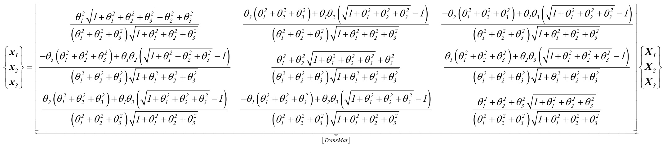
where [A] is referred to as the Bernoulli-Euler transformation matrix in this work. The approximation symbol (\approx) is used in place of an equals symbol (=) in the above expression since [A] is not orthonormal, which implies that the resulting \pmb{x} from this expression is not made up of a set of mutually orthogonal axes (all transformation matrices between sets of mutually orthogonal axes must be orthonormal). So it is evident that in place of [A] , what we want is the closest orthonormal matrix to [A] , which is referred to as \left[T r a n s M a t\right] in this work. From linear algebra, we know that the closest orthonormal matrix to [A] in the Frobenius Norm sense is:
\left[T r a n s M a t\right]{=}\left[U\right]\left[V\right]^{T},
where the columns of \left[U\right] contain the eigenvectors of \left[A\right]\!\!\left[A\right]^{T} and the columns of \big[V\big] contain the eigenvectors of \left[A\right]^{T}\left[A\right] . This result follows directly from the Singular Value Decomposition (SVD) of [A] :
[A]\!=\!\!\left[U\right]\!\!\left[\Sigma\right]\!\!\left[V\right]^{\scriptscriptstyle T},
where \left[\varSigma\right] is a diagonal matrix containing the singular values of [A] , which are \sqrt{e i g e n\nu a l u e s\;o f\left[A\right]\left[A\right]^{T}}\;=\sqrt{e i g e n\nu a l u e s\;o f\left[A\right]^{T}\left[A\right]}\;.
This was derived symbolically by J. Jonkman by computing \left[U\right]\!\!\left[V\right]^{T} by hand with verification in Mathematica.
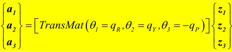
Tower Base / Platform Coordinate System
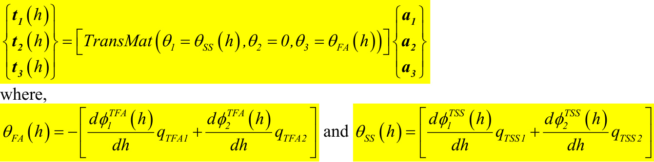
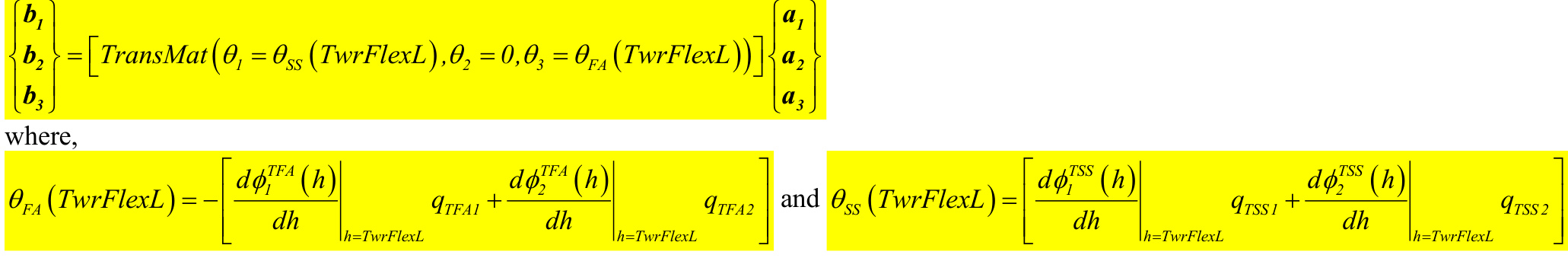
Tower Element-Fixed Coordinate System
Tower-Top / Base Plate Coordinate System
Nacelle / Yaw Coordinate System${\pmb d}{t}$ cos (qYaw) 0 −sin (qYaw) b${\pmb d}{2}$ 0 1 0 b${\pmb d}_{3}$ sin (qYaw) 0 cos (qYaw) b
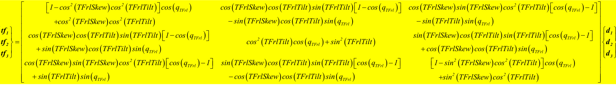
Rotor-Furl Coordinate System
<html>| -cos +COs rf RFrlSkew)cos rf2 +sin rf3 COS RFrlSkew)sin +sin RFrlTilt) | RFrlSkew)cos RFrlTilt RFrlSkew)cos COS 9RFrl COS RFrlSkew)cos RFrlTilt -sin RFrlSkew)cos RFrlTilt RFrlTilt 1-cos sin 9RFr! OS RFrlSkew)cos RFrlTilt sin 9RFr! RFrlSkew)cos RFrlTilt cos(qRFrl )- 1] sin RFrlSkew)cos sin 9RFrl RFrlSkew)cos | RFrlTilt sin RFrlTilt L 1-cos 9RFrl COS RFrlTilt sin -sin sin RFrlTilt )cos qRFrl +sin RFrlTilt +cOS RFrlTilt sin RFrlTilt COS )-1 RFrlTilt sin qRFrl | RFrlSkew)sin RFrlSkew)cos RFrlTilt )-1] qRFrl RFrlTilt )sin( 9RFrl RFrlSkew)cos RFrlTilt RFrlTilt -1 sin qRFrl d RFrlSkew)cos RFrlTilt sin 9RFrl 1-sin RFrlSkew)cos RFrlTilt COS 9RFrl +sin RFrlSkew)cos RFrlTilt |
Shaft Coordinate System
c_{I} cos (ShftSkew) cos (ShftTilt) sin (ShftTilt) −sin (ShftSkew) cos (ShftTilt) rf c_{2} cos (ShftSkew) sin (ShftTilt) cos (ShftTilt) sin (ShftSkew) sin (ShftTilt) c_{3} sin (ShftSkew) 0 cos (ShftSkew) rf3
Azimuth Coordinate System e_{I} 0 0 c_{I} e_{2} 0 cos (qDrTr+qGeAz) sin (qDrTr+qGeAz) c_{2} e 0 −sin (qDrTr+qGeAz) cos (qDrTr+qGeAz)
Teeter Coordinate System cos (qTeet 0 −sin (qTeet 0 1 0 sin (qTeet) 0 cos (qTeet)
Hub / Delta-3 Coordinate System
0
g_{I} 0 cos (Delta3) sin( Delta3)
g_{2}
\pmb{g}_{3} 0 −sin( Delta3) cos (Delta3)
Hub (Prime) Coordinate System
g'1B1 1 0 0 g1
g'2B1 = 0 1 0 g2
g B1 3 0 0 1 g3
The equation for {\pmb g}^{\,\circ\!B2} of blade 2 is similar.
Coned Coordinate System
<html>| B1 B1 2 B1 3 | PreCone (1)] PreCone (1)] sin | -sin 1 COS | PreCone ()]] PreCone (1)] | g B1 1 B1 g 2 g B1 3 |
The equation for i^{B2} is similar.
Blade / Pitched Coordinate System
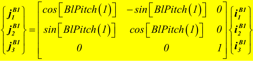
The equation for j^{B2} is similar.
Blade Coordinate System Aligned with Local Structural Axes (not element fixed)
Lj1B1(r ) cos θSB1(r ) −sinθSB1(r ) iB1
Lj2B1 (r ) θSB1(r ) cosθSB1(r ) B sin
\left\lfloor L j_{3}^{B I}\left(r\right)\right\rfloor B 0 0
The equation for L j^{B2}(r) is similar.
Blade Element-Fixed Coordinate System Aligned with Local Structural Axes
\begin{array}{r}{\left[n_{I}^{B I}\left(r\right)\right]}\\ {\left.\left|n_{2}^{B I}\left(r\right)\right\rangle=\left[T r a n s M a t\left(\theta_{I}=\theta_{x}^{B I}\left(r\right),\theta_{2}=\theta_{y}^{B I}\left(r\right),\theta_{3}=0\right)\right]\left[L j_{2}^{B I}\left(r\right)\right\rangle\right.}\\ {\left.\left|n_{3}^{B I}\left(r\right)\right\rangle\right]}\end{array}
where,
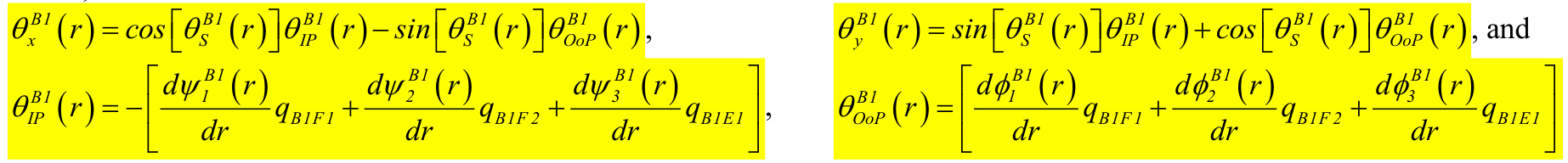
The equation for {\pmb n}^{B2}(r) is similar.
Blade Element-Fixed Coordinate System Used for Calculating and Returning Aerodynamic Loads This coordinate system is coincident with i^{B I} when the blade is undeflected.
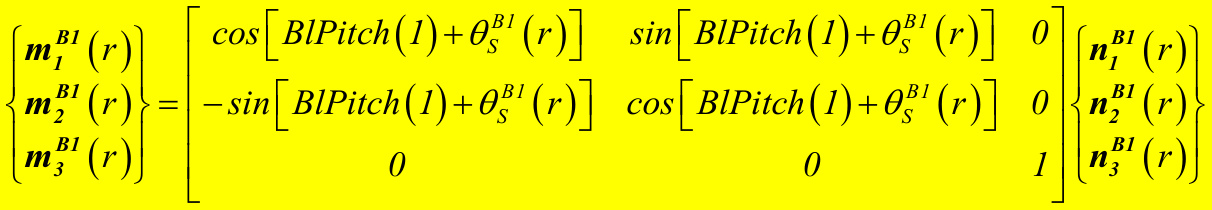
The equation for m^{B2}(r) is similar.
Blade Element-Fixed Coordinate System Aligned with Local Aerodynamic Axes (i.e., chordline) / Trailing Edge Coordinate System
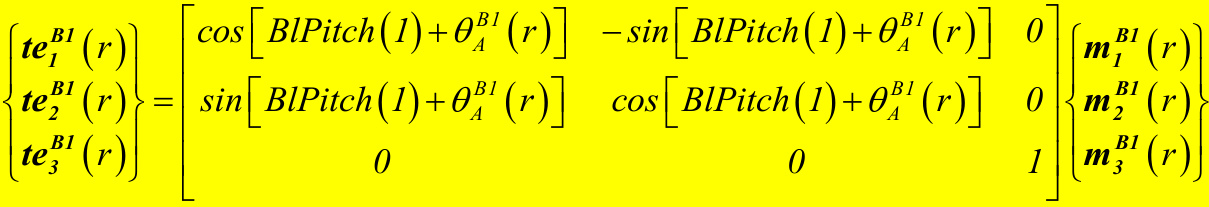
The equation for t e^{B2}(r) is similar.
Tail-Furl Coordinate System
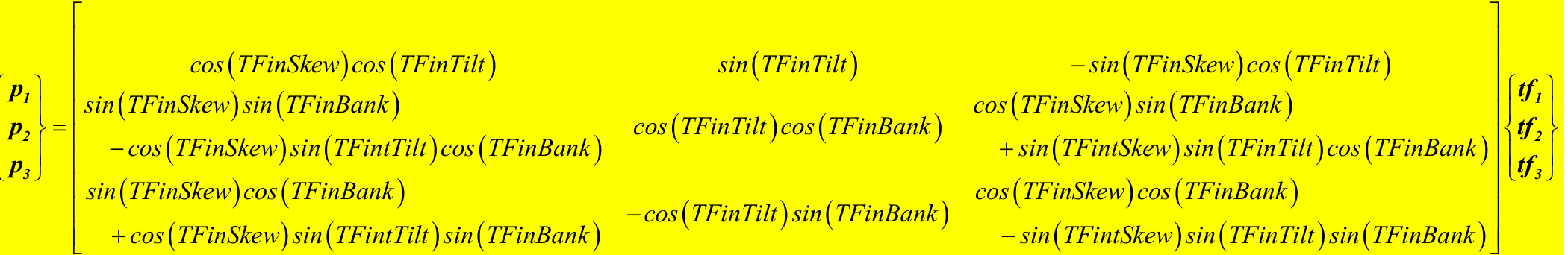
Tail Fin Coordinate System