# Implicit Floquet analysis of wind turbines using tangent matrices of a non-linear aeroelastic code  
利用非线性气弹耦合代码的切线矩阵进行风电机组的隐式Floquet分析

P. F. Skjoldan1 and M. H. Hansen2  

1 Loads, Aerodynamic and Control, Siemens Wind Power A/S, DK-2630 Taastrup, Denmark   
2 Wind Energy Division, National Laboratory for Sustainable Energy, Risø DTU, DK-4000 Roskilde, Denmark  

# ABSTRACT  

The aeroelastic code BHawC for calculation of the dynamic response of a wind turbine uses a non-linear finite element formulation. Most wind turbine stability tools for calculation of the aeroelastic modes are, however, based on separate linearized models. This paper presents an approach to modal analysis where the linear structural model is extracted directly from BHawC using the tangent system matrices when the turbine is in a steady state. A purely structural modal analysis of the periodic system for an isotropic rotor operating at a stationary steady state was performed by eigenvalue analysis after describing the rotor degrees of freedom in the inertial frame with the Coleman transformation. For general anisotropic systems, implicit Floquet analysis, which is less computationally intensive than classical Floquet analysis, was used to extract the least damped modes. Both methods were applied to a model of a three-bladed $2.3\;\mathrm{MW}$ Siemens wind turbine model. Frequencies matched individually and with a modal identification on time simulations with the non-linear model. The implicit Floquet analysis performed for an anisotropic system in a periodic steady state showed that the response of a single mode contains multiple harmonic components differing in frequency by the rotor speed. 
用于计算风电机组动态响应的空气弹性代码 BHawC 采用非线性有限元公式。然而，大多数用于计算空气弹性模态的风电机组稳定性工具仍然基于单独的线性化模型。本文提出了一种模态分析方法，该方法利用风电机组处于稳态时的切线系统矩阵，直接从 BHawC 中提取线性结构模型。通过描述惯性坐标系下的风轮自由度，并使用科尔曼变换，对各向同性风轮在固定稳态下的周期系统进行纯结构模态分析，采用特征值分析实现。对于一般的各向异性系统，采用隐式Floquet分析，其计算强度小于传统的Floquet分析，用于提取阻尼最小的模态。这两种方法都应用于一个三叶片 2.3 MW 西门子风电机组模型。特征频率与非线性模型的时间模拟模态识别结果相符。隐式Floquet分析表明，对于周期稳态下的各向异性系统，单个模态的响应包含多个频率不同的谐波分量，这些频率之差为风轮转速。

Copyright $\copyright$ 2011 John Wiley & Sons, Ltd.  

# KEYWORDS  

modal analysis; Floquet analysis; rotor dynamics  

# Correspondence  

P. F. Skjoldan, Loads, Aerodynamic and Control, Siemens Wind Power A/S, Dybendalsvænget 3, DK-2630 Taastrup, Denmark. E-mail: peter.skjoldan@siemens.com  

Received 26 June 2010; Revised 7 October 2010; Accepted 12 February 2011  

# 1. INTRODUCTION  

Today, advanced non-linear finite element codes1–3 are routinely used for load calculations on wind turbines. Most wind turbine stability tools for calculation of the aeroelastic modes are, however, based on separate linearized models. Stability analysis can be divided into three steps: first, a calculation of the steady state; then, a linearization of the equations of motion about the steady state and last, a modal analysis to extract modal frequencies, damping and mode shapes. This paper presents an approach to structural modal analysis applicable to any periodic steady state where the linearization is obtained directly from the non-linear wind turbine aeroelastic code BHawC.3  

The equations of motion for a wind turbine operating at a constant mean rotor speed contain periodic coefficients, preventing direct eigenvalue analysis of the system. Most recent wind turbine stability tools $4\mathrm{-}7$ incorporate the Coleman transformation, also known as the multiblade coordinate transformation, which describes the rotor degrees of freedom in the inertial frame. This transformation eliminates the periodic coefficients if the system is isotropic, i.e. the rotor consists of identical symmetrically mounted blades, and the environment conditions are symmetric. Floquet analysis is, however, applicable to anisotropic systems and any periodic steady state. It requires integration of the equations of motion over a period of rotor rotation, as many times as there are state variables in the system. Because of the computational burden of this approach, it has only been applied to reduce or simplify wind turbine models with a limited number of degrees of freedom.8–10 One way to reduce the computation time is to use the Fast Floquet Theory11 where only one third of the integrations are necessary for a three-bladed isotropic rotor. Another way is to use implicit Floquet analysis12 where the least damped modes can be extracted after a limited number of integrations.  

Stol et al.13 compare the Floquet analysis with the Coleman transformation approach applied to a periodic steady state, where the remaining periodic coefficients are eliminated by averaging and find small differences in modal frequencies and damping, concluding that it is not necessary to use Floquet analysis.  

Another approach to modal analysis is system identification,14–16 which operates on the response from numerical simulations or measurements, and no knowledge of the system equations is needed to extract the modal properties. The accuracy of the methods is, however, limited and depends on the chosen excitation.  

In this paper, tangent matrices for mass, damping and stiffness are extracted from the aeroelastic code BHawC. If the system is isotropic and the steady state is stationary, the Coleman transformation is applied before extracting the modal parameters by eigenvalue analysis. For an anisotropic system, implicit Floquet analysis is used for the modal analysis. When the system is isotropic, the response of a single mode contains a single harmonic component for tower degrees of freedom and up to three components for the blades. The response of a single mode in the anisotropic system on both blades and tower contains multiple harmonic components differing in frequency by the rotor speed.  

Section 2 of this paper describes the BHawC model, and Section 3 explains the methods for modal analysis, the Coleman transformation approach, the implicit Floquet analysis and also the partial Floquet analysis, a system identification technique. In Section 4, the methods are applied to a model of a wind turbine. Section 5 discusses the approaches, and Section 6 concludes the paper.  

今天，先进的非线性有限元代码1–3被常规地用于风电机组的载荷计算。然而，大多数用于计算气弹振模态的风电机组稳定性工具，仍然基于独立的线性化模型。**稳定性分析可以分为三个步骤：首先，计算稳态；然后，对稳态运动方程进行线性化；最后，进行模态分析以提取模态频率、阻尼和模态形状**。本文提出了一种适用于任何周期稳态的结构模态分析方法，该方法直接从非线性风电机组气弹振代码BHawC.3中获得线性化结果。

在恒定平均风轮转速下运行的风电机组的运动方程包含周期系数，这阻止了对系统的直接特征值分析。大多数最近的风电机组稳定性工具$4\mathrm{-}7$采用了科尔曼变换，也称为多叶坐标变换，它在惯性坐标系中描述了风轮的自由度。如果系统是各向同性的，即风轮由对称安装的相同叶片组成，并且环境条件对称，则该变换可以消除周期系数。然而，Floquet分析适用于各向异性系统和任何周期稳态。它需要对运动方程在风轮旋转一个周期内进行积分，积分次数等于系统状态变量的数量。由于这种方法的计算负担，它仅被用于减少或简化具有有限自由度的风电机组模型。8–10 一种减少计算时间的方法是使用快速Floquet理论11，对于三叶各向同性风轮，只需要进行三分之一的积分。另一种方法是使用隐式Floquet分析12，可以在有限次数的积分后提取最弱阻尼的模态。

Stol等人13将Floquet分析与应用于周期稳态的科尔曼变换方法进行比较，通过平均消除剩余的周期系数，发现模态频率和阻尼存在微小差异，得出结论：不需要使用Floquet分析。

模态分析的另一种方法是系统辨识14–16，它基于数值模拟或测量结果，无需了解系统方程即可提取模态特性。然而，这些方法的精度有限，并且取决于所选的激励。

在本文中，质量、阻尼和刚度的切线矩阵从气弹振代码BHawC中提取。如果系统是各向同性的，稳态是静态的，则在提取模态参数并通过特征值分析之前，应用科尔曼变换。对于各向异性系统，使用隐式Floquet分析进行模态分析。当系统是各向同性的时，单个模态的响应包含单个谐波分量，用于塔架自由度，对于叶片则包含多达三个分量。各向异性系统中的单个模态响应，对于叶片和塔架都包含多个谐波分量，这些分量在频率上不同，相差风轮转速。

本文第2节描述了BHawC模型，第3节解释了模态分析方法，科尔曼变换方法、隐式Floquet分析以及部分Floquet分析（一种系统辨识技术）。第4节将这些方法应用于风电机组模型。第5节讨论这些方法，第6节总结了本文。



# 2. STRUCTURAL MODEL  

The BHawC wind turbine aeroelastic code3 is based on a structural finite element model sketched in Figure 1, where the main structural parts, tower, nacelle, shaft, hub and blades, are modelled as two-node 12-degrees of freedom Timoshenko beam elements. The code uses a corotational formulation, where each element has its own coordinate system that rotates with the element. The elastic deformation is described in the element frame, whereas the movement of the element coordinate system accounts for rigid body motion. In this way, a geometrically non-linear model is obtained using linear finite elements.  

The configuration of the system, defined by nodal positions $\pmb{p}$ and orientations $\pmb q$ , nodal velocities $\dot{\pmb u}$ (of both positions and orientations) and nodal accelerations $\ddot{u}$ , must satisfy the equilibrium equation given in global coordinates as  

BHawC风电机组气弹振代码3基于图1所示的结构有限元模型，其中主要结构部件，塔架、机舱、主轴、轮毂和叶片，被建模为两节点12自由度Timoshenko梁单元。该代码采用corotational公式，其中每个单元拥有自己的坐标系，该坐标系随单元旋转。弹性变形在单元坐标系中描述，而单元坐标系的运动则考虑了刚体运动。 这样，就使用线性有限元获得了几何非线性模型。

系统的配置，由节点位置 $\pmb{p}$ 和姿态 $\pmb q$ ，节点速度 $\dot{\pmb u}$ （位置和姿态均包含）和节点加速度 $\ddot{u}$ 定义，必须满足以全局坐标表示的平衡方程。


$$
f_{\mathrm{iner}}(\boldsymbol{p},\boldsymbol{q},\dot{\boldsymbol{u}},\ddot{\boldsymbol{u}})+f_{\mathrm{damp}}(\boldsymbol{q},\dot{\boldsymbol{u}})+f_{\mathrm{int}}(\boldsymbol{p},\boldsymbol{q})=f_{\mathrm{ext}}
$$  

where $f_{\mathrm{iner}},f_{\mathrm{damp}},f_{\mathrm{int}}$ and $\pmb{f}_{\mathrm{ext}}$ are the inertial, damping, internal and external force vectors, respectively, and $\dot{\mathrm{O}}=\mathrm{d}/\mathrm{d}t$ denotes a time derivative. The inertial forces depend on the acceleration of the masses, the damping forces are given by viscous damping, the internal forces are due to elastic forces and the external forces contain the aerodynamic forces.17 To find  
其中，$f_{\mathrm{iner}}$、 $f_{\mathrm{damp}}$、 $f_{\mathrm{int}}$ 和 $\pmb{f}_{\mathrm{ext}}$ 分别为惯性力、阻尼力、内力以及外力矢量，且 $\dot{\mathrm{O}}=\mathrm{d}/\mathrm{d}t$ 表示时间导数。惯性力取决于质量的加速度，阻尼力由粘性阻尼给出，内力由弹性力引起，外力包含气动力。<sup>17</sup> 为了找到
![](images/8c6afcabcd9b46b013d0b9eaf1928f2d43001587902377b212d0d820be50f7d8.jpg)  
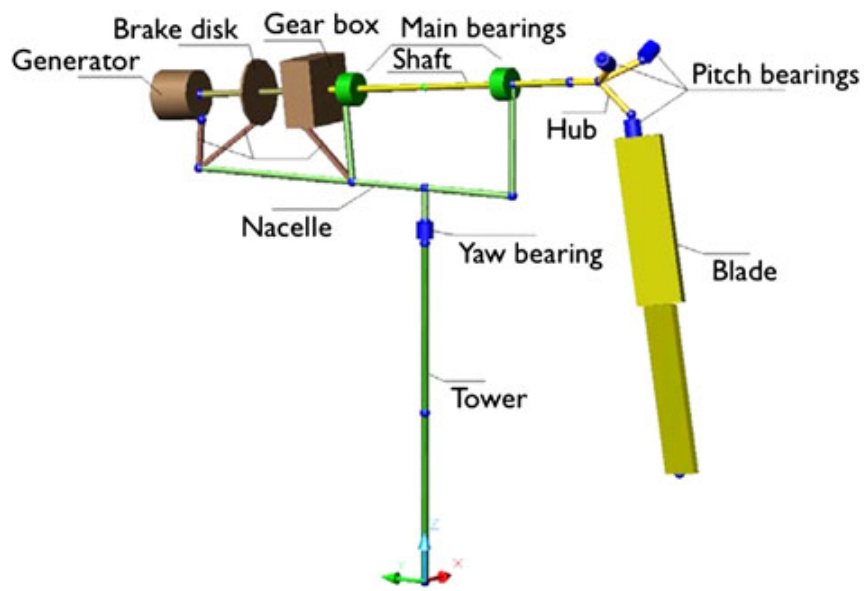
Figure 1. Sketch of the BHawC model substructures.  

this equilibrium configuration, increments of the positions and the orientations $\delta\pmb{u}$ , the velocities $\delta\dot{\pmb{u}}$ and the accelerations $\delta\ddot{\pmb{u}}$ are obtained using Newton–Raphson iteration with the tangent relation obtained from the variation of Equation (1) as  
这种平衡构型下，位置和姿态的增量 $\delta\pmb{u}$ 、速度 $\delta\dot{\pmb{u}}$ 和加速度 $\delta\ddot{\pmb{u}}$ 采用牛顿-拉夫逊迭代法获得，其切线关系式由方程 (1) 的变分推导得到，作为
$$
\mathbf{M}(q)\delta{\ddot{u}}+\mathbf{C}(q,{\dot{u}})\delta{\dot{u}}+\mathbf{K}(p,q,{\dot{u}},{\ddot{u}})\delta u=r
$$  

where M, C and $\mathbf{K}$ are the tangent mass, damping/gyroscopic and stiffness matrices, respectively, and $r=f_{\mathrm{ext}}+f_{\mathrm{iner}}+$ $f_{\mathrm{damp}}\!-\!f_{\mathrm{int}}$ is the residual. The stiffness matrix is composed of constitutive, geometric and inertial stiffness. The orientation $\pmb q$ of the nodes is described by quaternions, also known as the Euler parameters,18 a general four-parameter representation equivalent to a triad, which for node number $i$ is updated as  
其中 M、C 和 $\mathbf{K}$ 分别为切向质量、阻尼/陀螺和刚度矩阵，且 $r=f_{\mathrm{ext}}+f_{\mathrm{iner}}+$ $f_{\mathrm{damp}}\!-\!f_{\mathrm{int}}$ 为残余量。刚度矩阵由本构刚度、几何刚度和惯性刚度组成。节点方向 $\pmb q$，由四元数描述，也称为欧拉参数<sup>18</sup>，这是一种与三维坐标系等效的通用四参数表示，对于节点编号 $i$ 而言，其更新方式为：
$$
\pmb q_{i}:=q u a t(\delta\pmb u_{i,\mathrm{rot}})*\pmb q_{i}
$$  

where $\delta\mathbf{\boldsymbol{u}}_{i,\mathrm{rot}}$ contains three rotations that are assumed infinitesimal and thus commute and where this rotation pseudovector is transformed by the function termed quat into a quaternion, which is used to update the nodal quaternion $\pmb q_{i}$ employing the special quaternion product denoted by $^*$ , which maintains the unity of the quaternion. The nodal positions $\pmb{p}$ , the nodal velocities $\dot{\pmb u}$ and the accelerations $\ddot{u}$ are updated by regular addition of the positional part of $\delta\pmb{u},\,\delta\dot{\pmb{u}}$ and $\delta\ddot{\pmb{u}}$ , respectively. All components in $\pmb{p}$ , $\pmb q$ and $\delta\pmb{u}$ are absolute and described in a global frame.  

The present work considers small perturbations in position and orientation ${\bf\delta y}$ , velocity $\dot{\mathbf{y}}$ and acceleration $\ddot{\mathbf{y}}$ to a steady state with constant mean rotor speed $\varOmega$ defined by $(p_{\mathrm{ss}},q_{\mathrm{ss}},\dot{\pmb u}_{\mathrm{ss}},\ddot{\pmb u}_{\mathrm{ss}})$ , the steady state positions, orientations, velocities and accelerations, respectively, all periodic with the rotor period $T=2\pi/\varOmega$ . The linearized equations of motion are obtained from equation (2) at $r\approx\theta$ as  
其中 $\delta\mathbf{\boldsymbol{u}}_{i,\mathrm{rot}}$ 包含三个假设为无穷小的旋转，因此可以交换，并且这个旋转伪矢量通过称为“quat”的函数转换成一个四元数，用于更新节点四元数 $\pmb q_{i}$，采用特殊的四元数乘积（用 $^*$ 表示），该乘积保持四元数的模为一。节点位置 $\pmb{p}$ 、节点速度 $\dot{\pmb u}$ 和加速度 $\ddot{u}$ 分别通过正规地加回 $\delta\pmb{u}$、$\delta\dot{\pmb{u}}$ 和 $\delta\ddot{\pmb{u}}$ 的位置部分来更新。$\pmb{p}$、$\pmb q$ 和 $\delta\pmb{u}$ 中的所有分量都是绝对的，并且描述在全局坐标系中。

本工作考虑了位置和姿态 ${\bf\delta y}$ 、速度 $\dot{\mathbf{y}}$ 和加速度 $\ddot{\mathbf{y}}$ 在稳态下发生的微小扰动，稳态具有恒定的平均风轮转速 $\varOmega$，由 $(p_{\mathrm{ss}},q_{\mathrm{ss}},\dot{\pmb u}_{\mathrm{ss}},\ddot{\pmb u}_{\mathrm{ss}})$ 定义，分别代表稳态位置、姿态、速度和加速度，它们都具有风轮周期 $T=2\pi/\varOmega$ 。运动方程的线性化是通过在 $r\approx\theta$ 时从方程 (2) 获得的。


$$
{\bf M}({q}_{\mathrm{ss}})\ddot{\boldsymbol{y}}+{\bf C}({q}_{\mathrm{ss}},\dot{\boldsymbol{u}}_{\mathrm{ss}})\dot{\boldsymbol{y}}+{\bf K}({p}_{\mathrm{ss}},{q}_{\mathrm{ss}},\dot{\boldsymbol{u}}_{\mathrm{ss}},\ddot{\boldsymbol{u}}_{\mathrm{ss}}){\boldsymbol{y}}=\boldsymbol{\theta}
$$  

where the matrices $\mathbf{M}$ , $\mathbf{C}$ and $\mathbf{K}$ are the $T$ -periodic tangent system matrices that are employed in the modal analysis described in the next section.  
其中，矩阵 $\mathbf{M}$ 、 $\mathbf{C}$ 和 $\mathbf{K}$ 是在下一节中描述的模态分析中使用的 $T$ 周期切线系统矩阵。
# 3. METHODS  

In this section, the four methods for modal analysis of structures with rotors are presented.  
在本节中，将介绍四种带有风轮结构的模态分析方法。
# 3.1. Coleman approach  

The Coleman transformation requires identical degrees of freedom on each blade, and therefore, the equations of motion (equation (4)) in global coordinates were first transformed into substructure coordinates $y_{\mathrm{T}}$ . The transformation is  
科尔曼变换要求每个叶片具有相同的自由度，因此，首先将全局坐标系下的运动方程（方程(4)）转换到次结构坐标 $y_{\mathrm{T}}$ 。该变换是：


$$
\begin{array}{r l}&{\boldsymbol{y}=\mathrm{\mathbf{T}}\boldsymbol{y}_{\mathrm{T}}}\\ &{\mathbf{T}=\mathbf{diag}(\mathbf{I}_{N_{s}},\mathbf{T}_{\mathrm{r}},\mathbf{T}_{\mathrm{b1}},\mathbf{T}_{\mathrm{b2}},\mathbf{T}_{\mathrm{b3}})}\end{array}
$$  

where $\mathbf{T}$ is a block diagonal time-variant matrix composed of the identity matrix $\mathbf{I}_{N_{\mathrm{s}}}$ sized by the number of degrees of freedom of the tower, the nacelle and the drivetrain, $\mathbf{T_{r}}$ transforms the degrees of freedom on the shaft and the hub into a hub centre frame and $\mathrm{T}_{\mathfrak{b}j}$ transforms the degrees of freedom on blade number $j=1,2,3$ into a local frame for blade $j$ . The triads were obtained in the periodic steady state, and thus, $\mathbf{T}$ is $T$ -periodic.  

The time-variant transformation into inertial frame coordinates $z$ is  

其中，$\mathbf{T}$ 是一个块对角时间变动矩阵，由塔、机舱和传动系统自由度数量定义的单位矩阵 $\mathbf{I}_{N_{\mathrm{s}}}$ 组成，$\mathbf{T_{r}}$ 将主轴和轮毂的自由度变换到轮毂中心系，$\mathrm{T}_{\mathfrak{b}j}$ 将叶片编号 $j=1,2,3$ 的自由度变换到叶片 $j$ 的局部系。这些坐标系是在周期稳态下获得的，因此，$\mathbf{T}$ 是 $T$ 周期性的。

时间变动变换到惯性系坐标 $z$ 是
$$
\begin{array}{r l}&{{\mathbf y}_{\mathrm{T}}={\mathbf B}\,z}\\ &{{\mathbf B}={\textbf d i a g}({\mathbf I}_{N_{\mathrm{s}}},{\mathbf B}_{\mathrm{r}},{\mathbf B}_{\mathrm{b}})}\end{array}
$$  

where $\mathbf{B}_{\mathrm{r}}$ is a simple rotational transformation of the shaft and the hub and $\mathbf{B}_{\mathrm{b}}$ is the Coleman transformation introducing multiblade coordinates for a three-bladed rotor11,19 as  
其中 $\mathbf{B}_{\mathrm{r}}$ 是主轴和轮毂的一个简单旋转变换，而 $\mathbf{B}_{\mathrm{b}}$ 是科尔曼变换，它引入了三叶片风轮的多叶片坐标系<sup>11,19</sup>，如下所示：
$$
\mathbf{B}_{\mathrm{b}}=\left[\begin{array}{l l l}{\mathbf{I}_{N_{\mathrm{b}}}}&{\mathbf{I}_{N_{\mathrm{b}}}\cos\psi_{1}}&{\mathbf{I}_{N_{\mathrm{b}}}\sin\psi_{1}}\\ {\mathbf{I}_{N_{\mathrm{b}}}}&{\mathbf{I}_{N_{\mathrm{b}}}\cos\psi_{2}}&{\mathbf{I}_{N_{\mathrm{b}}}\sin\psi_{2}}\\ {\mathbf{I}_{N_{\mathrm{b}}}}&{\mathbf{I}_{N_{\mathrm{b}}}\cos\psi_{3}}&{\mathbf{I}_{N_{\mathrm{b}}}\sin\psi_{3}}\end{array}\right]
$$  

where $\psi_{j}=\varOmega t+2\pi(j-1)/3$ is the mean azimuth angle to blade number $j$ and $N_{\mathrm{b}}$ is the number of degrees of freedom on each blade. The inertial frame coordinate vector  
其中 $\psi_{j}=\varOmega t+2\pi(j-1)/3$ 是叶片序号 $j$ 的平均方位角，$N_{\mathrm{b}}$ 是每个叶片上的自由度数量。惯性坐标系向量
$$
\boldsymbol{z}=\{y_{\mathrm{s}}^{\mathrm{T}}\,z_{\mathrm{r}}^{\mathrm{T}}\,a_{0}^{\mathrm{T}}\,a_{1}^{\mathrm{T}}\,b_{1}^{\mathrm{T}}\}^{\mathrm{T}}
$$  

contains the untransformed coordinates for tower, nacelle and drivetrain ${\mathfrak{y}}_{\mathrm{s}}$ , the coordinates for shaft and hub $z_{\mathrm{r}}$ measured in a non-rotating frame aligned with the hub and the multiblade symmetric coordinates $\pmb{a}_{0}$ , cosine coordinates $\pmb{a}_{1}$ and sine coordinates $\pmb{b}_{1}$ . The details on how multiblade coordinates describe the motion of a wind turbine rotor in the inertial frame are discussed by Hansen.20,21  

The Coleman transformed equations were obtained by first inserting equation (5) into equation (4), then converting it to first order form and lastly introducing the inertial frame transformation in equation (6) as ${\displaystyle y_{\mathrm{T}2}=\mathrm{diag}({\bf B},{\bf B})z_{2}}$ where ${y}_{\mathrm{T}2}=\{{y}^{\mathrm{T}}\,{\dot{{y}}}^{\mathrm{T}}\}^{\mathrm{T}}$ and $z_{2}=\dot{\{z^{\mathrm{T}}\,\tilde{z}^{\mathrm{T}}\}}^{\mathrm{T}}$ are the state v ectors in substructure and ine rtial frames, respectively, with $\tilde{z}=\dot{z}+\bar{\omega}z$ and the constant matrix $\bar{\boldsymbol{\omega}}=\mathbf{B}^{-1}\mathbf{B}$ . The result is  
包含塔架、机舱和传动系统 ${\mathfrak{y}}_{\mathrm{s}}$ 的未转换坐标，主轴和轮毂 $z_{\mathrm{r}}$ 在与轮毂对齐的非旋转参考系中测量，以及多叶对称坐标 $\pmb{a}_{0}$，余弦坐标 $\pmb{a}_{1}$ 和正弦坐标 $\pmb{b}_{1}$。Hansen.20,21 讨论了多叶坐标如何描述风轮叶片在惯性参考系中的运动。

通过首先将方程(5)代入方程(4)，然后将其转换为一阶形式，最后引入方程(6)中的惯性参考系变换，获得了 Coleman 变换后的方程，形式为 ${\displaystyle y_{\mathrm{T}2}=\mathrm{diag}({\bf B},{\bf B})z_{2}}$，其中 ${y}_{\mathrm{T}2}=\{{y}^{\mathrm{T}}\,{\dot{{y}}}^{\mathrm{T}}\}^{\mathrm{T}}$ 和 $z_{2}=\dot{\{z^{\mathrm{T}}\,\tilde{z}^{\mathrm{T}}\}}^{\mathrm{T}}$ 分别是子结构和惯性参考系中的状态向量，且 $\tilde{z}=\dot{z}+\bar{\omega}z$，$\bar{\boldsymbol{\omega}}=\mathbf{B}^{-1}\mathbf{B}$ 为常数矩阵。结果为：
$$
\begin{array}{r l}&{\dot{z}_{2}=\mathbf{A}_{\mathrm{B}}z_{2}}\\ &{\mathbf{A}_{\mathrm{B}}=\left[\mathbf{-}\mathbf{\bar{\omega}}-\mathbf{\bar{\omega}}\mathbf{\bar{\omega}}_{\mathrm{KB}}\quad\mathbf{-M}_{\mathrm{B}}^{-1}\mathbf{C}_{\mathrm{B}}-\mathbf{\bar{\omega}}\right]}\end{array}
$$  

where $\mathbf{A}_{\mathrm{B}}$ is the Coleman transformed system matrix and  
其中 $\mathbf{A}_{\mathrm{B}}$ 是科尔曼变换后的系统矩阵，并且
$$
\begin{array}{r l}&{\mathbf{M}_{\mathrm{B}}=\mathbf{B}^{-1}\mathbf{T}^{\mathrm{T}}\mathbf{M}\mathbf{T}\,\mathbf{B}}\\ &{\mathbf{C}_{\mathrm{B}}=\mathbf{B}^{-1}\mathbf{T}^{\mathrm{T}}(\mathbf{C}\,\mathbf{T}+2\,\mathbf{M}\,\dot{\mathbf{T}})\mathbf{B}}\\ &{\mathbf{K}_{\mathrm{B}}=\mathbf{B}^{-1}\mathbf{T}^{\mathrm{T}}(\mathbf{K}\,\mathbf{T}+\mathbf{C}\,\dot{\mathbf{T}}+\mathbf{M}\,\ddot{\mathbf{T}})\mathbf{B}}\end{array}
$$  

are the Coleman transformed mass, damping/gyroscopic and stiffness matrices, respectively. If the system is isotropic, then $\mathbf{A}_{\mathrm{B}}$ is time-invariant, and a transient solution of equation (9) is  
分别是柯尔曼变换的质量、阻尼/陀螺和刚度矩阵。如果系统是各向同性，则 $\mathbf{A}_{\mathrm{B}}$ 是时不变的，方程 (9) 的瞬态解是
$$
z_{2}=\mathrm{e}^{\mathbf{A}_{\mathrm{B}}t}z_{2}(0)=\mathbf{V}\mathrm{e}^{\Lambda t}q(0)
$$  

where $\Lambda$ is a diagonal matrix containing the eigenvalues of $\mathbf{A}_{\mathrm{B}}$ , $\mathbf{V}$ contains the corresponding eigenvectors as columns and $\pmb q(0)=\mathbf V^{-1}z_{2}(0)$ are the initial conditions in modal coordinates. It is assumed that all eigenvectors are linearly independent .  

The blade motion given in the inertial frame in equation (11) can be transformed back into the rotating frame using equation (6) as $^{21}$  
其中 $\mathbf{A}$ 是包含 $\mathbf{A}_{\mathrm{B}}$ 特征值的对角矩阵，$\mathbf{V}$ 包含相应的特征向量作为列，且 $\pmb q(0)=\mathbf V^{-1}z_{2}(0)$ 是模态坐标下的初始条件。假设所有特征向量线性无关。

惯性坐标系中的叶片运动（见公式(11)）可以使用公式(6)转换回旋转坐标系，表示为 $^{21}$
$$
y_T,i k=\mathrm{e}^{\sigma_{k}t}\left(A_{0,i k}\cos(\omega_{k}t+\varphi_{0,i k})+A_{\mathrm{BW},i k}\cos\left((\omega_{k}+\Omega)t+\varphi_{j}+\varphi_{\mathrm{BW},i k}\right)+A_{\mathrm{FW},i k}\cos\left((\omega_{k}-\Omega)t-\varphi_{j}+\varphi_{\mathrm{GW},i k}\right)\right),
$$  

where $\varphi_{j}=2\pi(j-1)/3$ and $\sigma_{k}$ and $\omega_{k}$ pare the modal damping and frequency of mode number $k$ , respectively, given by the eigenvalue $\lambda_{k}=\sigma_{k}+\mathrm{i}\omega_{k}$ with $\mathrm{i}=\sqrt{-1}$ . The amplitudes for degree of freedom number $i$ were determined from the components of the eigenvector $\nu_{k}$ gi ven in multiblade coordinates of equation (8) as $A_{0,i k}=|a_{0,i k}|$ and  
其中 $\varphi_{j}=2\pi(j-1)/3$ ，$\sigma_{k}$ 和 $\omega_{k}$ 分别为模态阻尼和第 $k$ 个模态的频率，由特征值 $\lambda_{k}=\sigma_{k}+\mathrm{i}\omega_{k}$ 给出，其中 $\mathrm{i}=\sqrt{-1}$ 。自由度编号 $i$ 的振幅由方程 (8) 中多叶片坐标的特征向量 $\nu_{k}$ 的分量确定，为 $A_{0,i k}=|a_{0,i k}|$ 并且
$$
\begin{array}{r l}&{A_{\mathrm{BW},i k}=\frac{1}{2}\big((\mathrm{Re}\,(a_{1,i k})+\mathrm{Im}\,(b_{1,i k}))^{2}+(\mathrm{Re}\,(b_{1,i k})-\mathrm{Im}\,(a_{1,i k}))^{2}\big)^{1/2}}\\ &{A_{\mathrm{FW},i k}=\frac{1}{2}\big((\mathrm{Re}\,(a_{1,i k})-\mathrm{Im}\,(b_{1,i k}))^{2}+(\mathrm{Re}\,(b_{1,i k})+\mathrm{Im}\,(a_{1,i k}))^{2}\big)^{1/2}}\end{array}
$$  

where the subscripts 0, BW and FW denote symmetric, backward whirling and forward whirling motion, respectively.  
其中，下标 0、BW 和 FW 分别表示对称、后旋和前旋运动。
# 3.2. Classical Floquet analysis  

Floquet analysis enables the solution of the periodic equations of motion directly without an explicit transformation. Equation (4) is written in first order form  
Floquet 分析能够直接求解周期运动方程，无需显式变换。方程 (4) 以一阶形式写出。
$$
\begin{array}{r l}&{\dot{\boldsymbol{y}}_{2}=\mathbf{A}\boldsymbol{y}_{2}}\\ &{\mathbf{A}=\left[\mathbf{-M}^{-1}\mathbf{K}\quad\mathbf{-M}^{-1}\mathbf{C}\right]}\end{array}
$$  

where ${\mathbf y}_{2}=\{{\mathbf y}^{{\mathrm T}}\,\dot{{\mathbf y}}^{{\mathrm T}}\}^{{\mathrm T}}$ is the state vector and $\mathbf{A}$ is the $T$ -periodic system matrix.  

Floquet theory$^{22}$ states that the solution to equation (15) is of the form  
其中 ${\mathbf y}_{2}=\{{\mathbf y}^{{\mathrm T}}\,\dot{{\mathbf y}}^{{\mathrm T}}\}^{{\mathrm T}}$ 是状态向量，$\mathbf{A}$ 是 $T$ -周期系统矩阵。

Floquet理论$^{22}$ 指出，方程 (15) 的解具有如下形式：
$$
\mathbf{\boldsymbol{y}}_{2}=\mathbf{\boldsymbol{U}}\mathbf{\boldsymbol{e}}^{\mathbf{\boldsymbol{\Lambda}}t}\mathbf{\boldsymbol{U}}^{-1}(0)\mathbf{\boldsymbol{y}}_{2}(0)
$$  

where $\mathbf{U}$ is a $T$ -periodic matrix and $\mathbf{A}$ is a diagonal matrix. One way to construct this solution is to form a fundamental solution to equation (15) as  
其中 $\mathbf{U}$ 是一个 $T$ 周期矩阵，而 $\mathbf{A}$ 是一个对角矩阵。一种构造该解的方法是构造方程 (15) 的基本解，如下所示：
$$
\displaystyle\varphi=\bigl[\varphi_{1}\quad\varphi_{2}\quad.\ .\quad\varphi_{N}\bigr]
$$  

over one period, $t\ \in\ [0;T]$ , where $N$ is the number of state variables, such that $\dot{\varphi}\;=\;{\bf A}\varphi$ . The monodromy matrix defined as  
在周期内，$t\ \in\ [0;T]$ ，其中 $N$ 为状态变量的数量，且 $\dot{\varphi}\;=\;{\bf A}\varphi$ 。单值性矩阵定义为：
$$
\mathbf{C}=\boldsymbol{\varphi}^{-1}(0)\boldsymbol{\varphi}(T)
$$  

contains all modal properties, which can be extracted from the eigenvalue decomposition  
包含所有模态特性，可通过特征值分解提取。
$$
\mathbf{C}=\mathbf{V}\mathbf{J}\mathbf{V}^{-1}
$$  

where $\mathbf{V}$ contains the column eigenvectors $\nu_{k}$ of $\mathbf{C}$ , which are all assumed to be linearly independent and $\mathbf{J}$ is a diagonal matrix containing the eigenvalues $\rho_{k}$ of $\mathbf{C}$ , called the characteristic multipliers. The characteristic exponents $\lambda_{k}=\sigma_{k}+\mathrm{i}\omega_{k}$ contain the frequency $\omega_{k}$ and damping $\sigma_{k}$ and are related to the characteristic multipliers as $\rho_{k}=\exp(\lambda_{k}T)$ . Because the complex logarithm is not unique, the frequency is not determined uniquely, and the principal frequency $\omega_{\mathrm{p},k}$ and the damping $\sigma_{k}$ are defined from the characteristic multipliers as  
其中 $\mathbf{V}$ 包含矩阵 $\mathbf{C}$ 的列特征向量 $\nu_{k}$，假设它们线性无关，而 $\mathbf{J}$ 是一个对角矩阵，包含矩阵 $\mathbf{C}$ 的特征值 $\rho_{k}$，称为特征乘数。特征指数 $\lambda_{k}=\sigma_{k}+\mathrm{i}\omega_{k}$ 包含频率 $\omega_{k}$ 和阻尼 $\sigma_{k}$，并且与特征乘数相关，关系为 $\rho_{k}=\exp(\lambda_{k}T)$。由于复数对数不唯一，频率不能唯一确定，因此从特征乘数定义了主频率 $\omega_{\mathrm{p},k}$ 和阻尼 $\sigma_{k}$。
$$
\begin{array}{c}{\displaystyle\sigma_{k}=\frac{1}{T}\ln(\vert\rho_{k}\vert)}\\ {\displaystyle\omega_{\mathrm{p},k}=\frac{1}{T}\arg(\rho_{k})}\end{array}
$$  

where $\arg(\rho_{k})\in\big[-\pi;\pi]$ is implied, resulting in $\omega_{\mathrm{p},k}\in\big[-\Omega/2;\Omega/2\big]$ . Any integer multiple of the rotor speed can be added to the principal frequency to obtain a more physically meaningful frequency23,24  
其中隐含条件为 $\arg(\rho_{k})\in\big[-\pi;\pi]$，由此得出 $\omega_{\mathrm{p},k}\in\big[-\Omega/2;\Omega/2\big]$。 可以将风轮转速的任意整数倍加到主频上，以获得更具物理意义的频率²³，²⁴
$$
\omega_{k}=\omega_{\mathrm{p},k}+j_{k}\Omega
$$  

a choice that also affects the periodic modal matrix $\mathbf{U}$ in equation (16). This matrix $\mathbf{U}$ contains the periodic mode shapes uk and is given as24  
一个也会影响方程(16)中的周期模态矩阵 $\mathbf{U}$ 的选择。该矩阵 $\mathbf{U}$ 包含周期模态形状 uk，其表达式为24。

$$
\pmb{u}_{k}=\varphi\nu_{k}\mathrm{e}^{-\lambda_{k}t}
$$  

where the real part of $\lambda_{k}$ is given by equation (20) and the imaginary part of $\lambda_{k}$ is defined by equation (21) by selecting $j_{k}$ such that $\pmb{u}_{k}$ is as constant as possible for degrees of freedXom measured in the inertial frame.  

Introducing the Fourier transform of the periodic mode shape  
其中，$\lambda_{k}$ 的实部由公式(20)给出，虚部由公式(21)定义，通过选择 $j_{k}$ 使得在惯性坐标系测量的自由度方向上，$\pmb{u}_{k}$ 尽可能恒定。

引入周期模态的傅里叶变换
$$
{\pmb u}_{k}=\sum_{j=-\infty}^{\infty}u_{j k}\mathrm{e}^{\mathrm{i}j\Omega t}
$$  

the transient solution in equation (16) can be written as a sum of harmonic components  
方程 (16) 中的瞬态解可以写成谐波分量的和。
$$
y_{2}=\sum_{k=1}^{N}\sum_{j=-\infty}^{\infty}\mathcal{U}_{j k}\mathrm{e}^{(\sigma_{k}+\mathrm{i}(\omega_{k}+j\Omega))t}q_{k}(0)
$$  

where $\begin{array}{r}{\pmb q(0)=\mathbf{U}^{-1}(0)\mathbf{y}_{2}(0).}\end{array}$ . Note that equation (12) is a special case of this expression for $j=-1,0,1$  
其中 $\begin{array}{r}{\pmb q(0)=\mathbf{U}^{-1}(0)\mathbf{y}_{2}(0).}\end{array}$ 。 注意，当 $j=-1,0,1$ 时，方程 (12) 是此表达式的一个特例。
# 3.3. Implicit Floquet analysis  

The implicit Floquet method is here described based on the detailed description in Bauchau and Nikishkov,12 which focuses on computation of the characteristic multipliers from the state transition matrix $\Phi(T,0)$ . It can be defined in classical Floquet theory as  
基于Bauchau和Nikishkov的详细描述，本文介绍隐式Floquet方法，重点在于从状态转移矩阵$\Phi(T,0)$计算特征乘数。它可在经典Floquet理论中定义为：


$$
\boldsymbol{\varphi}(T)=\boldsymbol{\Phi}(T,0)\,\boldsymbol{\varphi}(0)
$$  

Using equation (18), the relationship between the state transition and monodromy matrices is derived as  
使用公式(18)，推导了状态转移矩阵与单值性矩阵之间的关系。
$$
\Phi(T,0)=\varphi(0){\bf C}\,\varphi^{-1}(0)
$$  

showing that $\Phi(T,0)$ and C have identical eigenvalues (characteristic multipliers), and their eigenvectors are related as $\pmb{\nu}_{k}=\pmb{\varphi}^{-1}(0)\pmb{w}_{k}$ , where $w_{k}$ represents the eigenvectors of $\Phi(T,0)$ .  
表明 $\Phi(T,0)$ 和 C 具有相同的特征值（特征乘数），且它们的特征向量之间存在如下关系：$\pmb{\nu}_{k}=\pmb{\varphi}^{-1}(0)\pmb{w}_{k}$ ，其中 $\pmb{w}_{k}$ 代表 $\Phi(T,0)$ 的特征向量。
The key feature of the state transition matrix is that it defines the solution $y_{2}(T)=\Phi(T,0)y_{2}(0)$ for a time integration of the system equations (equation (15)) over one period $T$ with initial conditions ${\mathfrak{y}}_{2}(0)$ . Hence, without knowing the state transition matrix, it is possible to obtain the product of it with an arbitrary vector (the initial state vector) by integration of  
关键在于状态转移矩阵定义了系统方程（式(15)）在周期 $T$ 内的时间积分解 $y_{2}(T)=\Phi(T,0)y_{2}(0)$，初始条件为 ${\mathfrak{y}}_{2}(0)$。因此，在不知道状态转移矩阵的情况下，可以通过积分来获得它与任意向量（初始状态向量）的乘积。


equation (15) over one period. The Arnoldi algorithm25 is a method to approximate the eigenvalues and the eigenvectors of a matrix, say $\Phi(T,0)$ , using only the matrix multiplication with $\Phi(T,0)$ to construct an $m$ -sized subspace  
方程 (15) 描述了一个周期内的状态。Arnoldi算法²⁵是一种近似矩阵（例如 $\Phi(T,0)$ ）的特征值和特征向量的方法，仅通过与 $\Phi(T,0)$ 的矩阵乘法构建一个 $m$ 维子空间。
$$
\mathbf{P}=\left[p_{1}\quad p_{2}\quad\ldots\quad p_{m}\right]
$$  

that satisfies the orthonormality condition  

$$
\mathbf{P}^{\mathrm{T}}\mathbf{P}=\mathbf{I}
$$  

and where the eigenvalues $\tilde{\rho}_{k}$ of the subspace projected state transition matrix  

$$
\mathbf{H}=\mathbf{P}^{\mathrm{T}}\Phi(T,0)\mathbf{P}
$$  

converge towards the eigenvalues $\rho_{k}$ of $\Phi(T,0)$ with the largest modulus as the size $m$ of the subspace increases. The subspace eigenvectors $\tilde{w}_{k}$ of $\mathbf{H}$ projected back to the full state space converge towards the eigenvectors $w_{k}$ of $\Phi(T,0)$ , i.e. $w_{k}\approx\mathbf{P}\tilde{w}_{k}$ . The Arnoldi algorithm proceeds as follows:  

随着子空间维数 $m$ 的增大，子空间特征向量 $\tilde{w}_{k}$ 投影回完整状态空间，会收敛于 $\Phi(T,0)$ 的特征向量 $w_{k}$，即 $w_{k}\approx\mathbf{P}\tilde{w}_{k}$。阿诺尔迪算法的步骤如下：
Choose an arbitrary vector $\pmb{p}_{1}$ with $|p_{1}|=1$ for $n=1,2,\ldots,m$ 
$\pmb{a}:=\Phi(T,0)p_{n}$ (integration of equation (15) over $t\in[0;T])$ 
$\begin{array}{l}{b:=a}\\ {\mathrm{for~}j=1,2,\dotsc,n}\\ {\quad h_{j,n}:=p_{j}^{\operatorname{T}}a}\\ {\quad b:=b-h_{j,n}p_{j}}\end{array}$ 
end 
if $n<m$ $\begin{array}{l}{{h_{n+1,n}:=|b|}}\\ {{p_{n+1}:=b/h_{n+1,n}}}\end{array}$ 
end 
$\begin{array}{r}{p_{n+1}:=\!p_{n+1}-\!\sum_{j=1}^{n}\!(p_{j}^{\mathrm{T}}\!p_{n+1})p_{j}}\end{array}$ 
end  

The last step in the $n$ -loop is an explicit re-orthogonalization to eliminate an otherwise progressing skewness of the subspace basis and thereby ensure convergence of the algorithm.12 Note that $\mathbf{H}$ with components $h_{j,n}$ , $n\,=\,1,\dots,m$ , $j=1,\dots,n$ , is an upper Hessenberg matrix for which there exist efficient eigenvalue solvers. In practice, the Arnoldi algorithm is continued until a desired number of eigenvalues $\tilde{\lambda}_{k}$ with the largest modulus and their corresponding eigenvectors $\mathbf{P}\tilde{{\boldsymbol{w}}}_{k}$ of the state transition matrix $\Phi(T,0)$ are converged to within a specific tolerance.  

To construct the approximations to the periodic mo de shapes (equation (22)), the $m\times m$ fundamental solution matrix $\tilde{\varphi}$ to the subspace projected system equations is written as  
最后一步是显式地重新正交化，以消除否则会逐渐累积的子空间基底的偏斜，从而确保算法的收敛。12 注意，$\mathbf{H}$ 具有分量 $h_{j,n}$ ，$n\,=\,1,\dots,m$ ，$j=1,\dots,n$ ，是一个Hessenberg矩阵，存在高效的特征值求解器。在实践中，阿诺尔迪算法会持续进行，直到收敛到期望数量的具有最大模值的特征值 $\tilde{\lambda}_{k}$ 及其对应于状态转移矩阵 $\Phi(T,0)$ 的特征向量 $\mathbf{P}\tilde{{\boldsymbol{w}}}_{k}$，并且在特定容差范围内。

为了构造周期模态形状（方程 (22)）的近似值，将投影到子空间的系统方程的 $m\times m$ 基础解矩阵 $\tilde{\varphi}$ 写作：
$$
{\tilde{\boldsymbol{\varphi}}}=\mathbf{P}^{\mathrm{T}}\left[\varphi_{1}\quad\varphi_{2}\quad\ldots\quad\varphi_{m}\right]
$$  

where $\varphi_{j}$ is the solution of the full system (equation (15)) integrated over $t\in[0;T]$ for each initial condition $p_{j}$ , whereby ${\tilde{\boldsymbol{\varphi}}}(0)=\mathbf{I}$ because of equation (28). The eigenvectors $\tilde{\nu}_{k}$ of the subspace projected monodromy matrix $\tilde{\mathbf{C}}=\tilde{\boldsymbol{\Phi}}^{-1}(0)\tilde{\boldsymbol{\Phi}}(T)$ are therefore identical to the eigenvectors $\tilde{w}_{k}$ of the subspace projected state transition matrix (equation (29)). The periodic mode shapes in the subspace are therefore similar to equation (22) given by  
其中 $\varphi_{j}$ 是对每个初始条件 $p_{j}$ 在 $t\in[0;T]$ 积分得到的完整系统（方程 (15)）的解，由于方程 (28)，${\tilde{\boldsymbol{\varphi}}}(0)=\mathbf{I}$。因此，子空间投影单值性矩阵 $\tilde{\mathbf{C}}=\tilde{\boldsymbol{\Phi}}^{-1}(0)\tilde{\boldsymbol{\Phi}}(T)$ 的特征向量 $\tilde{\nu}_{k}$ 与子空间投影状态转移矩阵（方程 (29)）的特征向量 $\tilde{w}_{k}$ 相同。因此，子空间中的周期模态形状与方程 (22) 相似，由...
$$
\tilde{\b u}_{k}=\tilde{\b\varphi}\tilde{\b w}_{k}\mathrm{e}^{-\tilde{\lambda}_{k}t}
$$  

which by projection back into the full state spac e using $\pmb{u}_{k}=\pmb{\mathrm{P}}\tilde{\pmb{u}}_{k}$ y ields the approximated periodic mode shapes of the full system  

$$
\boldsymbol{u}_{k}\approx\left[\varphi_{1}\quad\varphi_{2}\quad.\dots\quad\varphi_{m}\right]\tilde{w}_{k}\mathrm{e}^{-\tilde{\lambda}_{k}t}
$$  

where $\tilde{w}_{k}$ and $\tilde{\lambda}_{k}$ are the eigenvectors and characteristic exponents of $\mathbf{H}$ , respectively.  

# 3.4. Partial Floquet analysis  

Partial Floquet analysis23 is a system identification technique that operates on signals with the free response of the system, thus no knowledge of the system equations is necessary. The signals can be obtained by numerical simulation or from measurements.  

Singular value decomposition is used to eliminate noise and extract the frequency and the damping of the most dominant modes from a matrix similar to the monodromy matrix assembled from a limited number of signals spanning several periods. The entries in this matrix can only be sampled once per period for periodic systems, which limits the accuracy because the signal damps away, decreasing the signal to noise ratio. Time-invariant systems can, however, be sampled once per time step. Therefore, partial Floquet analysis is combined with Coleman transformation of the signals,26 such that the response resembles that of a time-invariant system. This approach increases the accuracy and the number of modes that can be extracted from a given signal. However, a careful choice of forcing that excites all modes of interest to a sufficient level is necessary to extract these modes accurately.  

部分Floquet分析23是一种系统识别技术，它基于系统的自由响应信号进行操作，因此无需了解系统方程。这些信号可以通过数值模拟或测量获得。

利用奇异值分解来消除噪声，并从一个类似于由有限数量的信号组装而成的单值矩阵中提取最主要的模态的频率和阻尼。对于周期系统，该矩阵中的元素每周期只需采样一次，这会限制精度，因为信号会衰减，降低信噪比。然而，时不变系统可以每时间步采样一次。因此，部分Floquet分析与信号的科尔曼变换相结合26，使得响应类似于时不变系统的响应。这种方法提高了精度，并增加了可以从给定信号中提取的模态数量。然而，为了准确提取这些模态，需要仔细选择能够以足够的水平激发所有感兴趣模态的激励。



# 4. NUMERICAL RESULTS  

The modal analysis methods described in the previous sections are applied to a BHawC model of a $2.3\;\mathrm{MW}$ wind turbine with three $45\;\mathrm{m}$ blades, hub height $80\;\mathrm{m}$ and nominal speed $16\,\mathrm{rpm}$ . The model has 381 structural degrees of freedom.  
前几节描述的模态分析方法应用于一个$2.3\;\mathrm{MW}$风电机组的BHawC模型，该风电机组具有三片$45\;\mathrm{m}$叶片，塔顶高度$80\;\mathrm{m}$，标称转速$16\,\mathrm{rpm}$。该模型包含381个结构自由度。
# 4.1. Isotropic system  

The turbine is mounted with identical blades and runs in a vacuum neglecting gravity forces, so the system is isotropic. The deflection of the blades because of centrifugal forces is therefore constant in the blade frame. The constant steady state is found at a given azimuth position by solving equation (1) statically, including centrifugal forces from the constant rotor speed. In this way, a steady state with no transients is obtained, and the system matrices become exactly periodic.  
机组安装有完全相同的叶片，并在忽略重力作用的真空环境中运行，因此系统各向同性。由于离心力引起的叶片变形在叶片坐标系中是恒定的。通过静态求解方程（1），包括恒定风轮转速引起的离心力，可以在给定的方位角位置找到稳定的稳态。 这样可以获得无瞬态的稳态，并且系统矩阵变得精确的周期性。
# 4.1.1. Coleman transformation approach  

Because the system is isotropic, a modal analysis can be performed on the Coleman transformed system matrix. The system matrices M, C and $\mathbf{K}$ from equation (4) were extracted at a single azimuth angle and combined into the Coleman transformed system matrix of equation (9) from which the modal frequencies, damping and eigenvectors given in the inertial frame were extracted. The time-invariance of the system matrix was checked by calculation for several azimuth angles.  

Figure 2(a) shows the lowest modal frequencies as a function of rotor speed where the frequency is normalized with the lowest modal frequency at $0\;\mathrm{rpm}$ . The modes were named according to their dominant motion determined from the eigenvector and the whirling amplitudes calculated from equations (13) and (14). The mode labels in Figure 2 first contain the index of that particular mode, then ‘T’ for tower, ‘F’ for blade flapwise, ‘E’ for blade edgewise or ‘DRV’ for drivetrain and ‘LO’ for longitudinal, ‘LA’ for lateral, ‘BW’ for backward whirling, ‘FW’ for forward whirling or $\mathbf{\nabla}^{\bullet}\mathbf{S}^{\bullet}$ for symmetric. For comparison, the frequencies extracted from time simulations with the non-linear BHawC model using the partial Floquet method26 are also shown. The agreement is within $0.4\%$ except for modes coupling to the drivetrain, i.e. the drivetrain, edgewise and lateral tower modes, where the discrepancy is up to $2\%$ at the highest rotor speed, which is caused by a difficulty with keeping the rotor speed exactly constant in the non-linear simulation because of the energy dissipated in the oscillation.  

由于系统具有各向同性，因此可以在科尔曼变换后的系统矩阵上进行模态分析。从方程(4)中提取的系统矩阵M、C和$\mathbf{K}$，在单个方位角下组合成方程(9)中的科尔曼变换后的系统矩阵，从中提取了在惯性坐标系下的模态频率、阻尼和特征向量。通过计算，验证了系统矩阵的时间不变性，在多个方位角下进行验证。

图2(a)显示了最低模态频率随风轮转速的变化曲线，频率以$0\;\mathrm{rpm}$时的最低模态频率为归一化值。模态的命名根据特征向量确定的主要运动和从方程(13)和(14)计算出的旋摆振幅来确定。图2中的模态标签首先包含该特定模态的索引，然后是‘T’代表塔架，‘F’代表叶片挥舞，‘E’代表叶片摆振，或‘DRV’代表机组，以及‘LO’代表纵向，‘LA’代表横向，‘BW’代表反向旋摆，‘FW’代表正向旋摆，或$\mathbf{\nabla}^{\bullet}\mathbf{S}^{\bullet}$代表对称模态。为了比较，还显示了使用部分Floquet方法26，从非线性BHawC模型的时间模拟中提取的频率。除了耦合到机组的模态（即机组、摆振和横向塔架模态）之外，一致性在0.4%以内，在最高风轮转速下，差异可达2%，这是由于在非线性模拟中，由于振荡过程中耗散的能量，难以保持风轮转速完全恒定。
![](images/995c2b6f3ee06ebcc2b34049a2242af9692ede73f9a2353ed42d793443f8df71.jpg)  
Figure 2. Frequency (a) and damping (b) as a function of rotor speed. Standstill eigenvalue analysis (squares), Coleman approach (lines), partial Floquet analysis (circles). Legend entries are ordered after the sequence at 0 rpm.  
图2. 转轮转速函数下的频率 (a) 和阻尼 (b)。静止特征值分析（方块），科尔曼法（线），偏分福克分析（圆）。图例条目按0 rpm时的顺序排列。

Figure 2(b) shows the damping as a function of rotor speed where the logarithmic decrement is normalized with the value for the first tower longitudinal mode at $0\;\mathrm{rpm}$ . The agreement in damping between the results from the linear model and the partial Floquet analysis applied to the non-linear model is within $6\%$ , except for a discrepancy of up to $20\%$ for modes coupling to the drivetrain. It must be noted that the purely structural damping of the modes is small, and thus, a small absolute difference leads to a high relative difference. The results also show that damping is more difficult to estimate than frequency using system identification.  
图 2(b) 显示了阻尼随风轮转速的变化，其中对第一塔纵向简正模态在 $0\;\mathrm{rpm}$ 时的对数衰减量进行了归一化。线性模型的结果与应用于非线性模型的偏Floquet分析结果在阻尼方面的吻合度在 $6\%$ 以内，除了与驱动系耦合的模态，存在高达 $20\%$ 的偏差。需要注意的是，这些模态的纯结构阻尼较小，因此，小的绝对差异会导致大的相对差异。结果还表明，与频率相比，系统辨识法更难估计阻尼。
# 4.1.2. Implicit Floquet analysis  

For the implicit Floquet analysis, the system matrices in global coordinates in equation (4) were extracted from the steady state at 16 azimuth angles equally spaced over a rotor rotation. For interpolation to other azimuth angles, a least squares fit of a truncated Fourier series with eight terms was used. The fundamental solutions in equation (30) were integrated with a Newmark-type solver from initial conditions determined by the Arnoldi algorithm. The principal frequencies and damping were found from equation (20) where $\rho_{k}$ are taken as the eigenvalues of the approximated state transition matrix. Figure 3 shows the real part $\sigma_{k}$ of the characteristic exponents calculated at each Arnoldi step for a steady state at $12\;\mathrm{rpm}$ using a time step of $\Delta t=T/1024=0.0049\;\mathrm{s}$ . The scattering of the highest damping values shows that the highest damped modes are spurious and do not represent actual eigenmodes of the system because of the approximate nature of the implicit Floquet analysis. To exclude these modes from the results, only modes satisfying a strict convergence criterion, where the absolute change of both damping $\sigma_{k}$ and principal frequency $\omega_{\mathrm{p},k}$ is less than $10^{-10}$ between three successive steps, were retained. After 50 Arnoldi steps, 19 modes were converged. The modal frequencies were determined using equation (21) by adding $j_{k}\Omega$ to the principal frequency, where $j_{k}\Omega$ is the single non-vanishing harmonic component in a Fourier transform of the periodic mode shape for degrees of freedom on the tower calculated from equation (32) using the principal frequency $\omega_{\mathrm{p},k}$ . The periodic mode shape components for degrees of freedom on the tower and the nacelle calculated with the modal frequency $\omega_{k}$ are thus constant. A detailed description of the process of frequency identification is given by Skjoldan and Hansen.24  

Figure 4 shows the difference in frequency calculated with the Coleman transformation approach and the implicit Floquet analysis with different integration time steps. The implicit Floquet results converge towards the Coleman transformation results for decreasing time steps, the error being roughly proportional to $\varDelta t^{2}$ . Predominantly, the error increases with the modal frequency. A similar trend is seen for the damping.  
为了进行隐式Floquet分析，方程(4)中的全局坐标系矩阵从风轮在16个方位角上均匀分布的稳态解中提取。为了插值到其他方位角，使用了截断的傅里叶级数，包含八个项，并采用最小二乘法拟合。方程(30)中的基本解使用Newmark型求解器，初始条件由Arnoldi算法确定。主频率和阻尼可以通过方程(20)得到，其中$\rho_{k}$被认为是近似状态转移矩阵的特征值。图3显示了在每个Arnoldi步计算得到的特征指数的实部$\sigma_{k}$，稳态转速为$12\;\mathrm{rpm}$，时间步长为$\Delta t=T/1024=0.0049\;\mathrm{s}$。最高阻尼值的散布表明，最高的阻尼模态是虚假的，由于隐式Floquet分析的近似性，它们不代表系统的实际特征模态。为了将这些模态从结果中排除，仅保留满足严格收敛判据的模态，即三个连续步长之间阻尼$\sigma_{k}$和主频率$\omega_{\mathrm{p},k}$的绝对变化均小于$10^{-10}$。经过50个Arnoldi步，19个模态收敛。模态频率使用方程(21)确定，通过将$j_{k}\Omega$加到主频率上，其中$j_{k}\Omega$是塔架自由度上周期模态的傅里叶变换中的单个非零谐波分量，该分量由方程(32)计算，并使用主频率$\omega_{\mathrm{p},k}$。因此，使用模态频率$\omega_{k}$计算出的塔架和机舱自由度上的周期模态分量是恒定的。Skjoldan和Hansen.24 详细描述了频率识别的过程。

图4显示了使用Coleman变换方法和隐式Floquet分析计算出的频率差，使用了不同的积分时间步长。随着时间步长的减小，隐式Floquet结果趋近于Coleman变换结果，误差大致与$\varDelta t^{2}$成正比。主要趋势是误差随着模态频率的增加而增加。阻尼也呈现出类似的趋势。


![](images/d300c31577c207a813cae8b5b1a3dc8e8c0459cc32696c8195e9ce09628530b1.jpg)  
Figure 3. Magnitude of implicit Floquet characteristic multipliers as function of steps in Arnoldi algorithm.   non-converged eigenvalues, $^{\circ}$ converged eigenvalues.  

![](images/07c41f3c180a256f6fc9f73409fcbda2a0ec65ee3d49fe15a72a2e4a7eda815d.jpg)  
Figure 4. Relative difference in implicit Floquet frequency compared with Coleman approach frequency for selected modes as a function of implicit Floquet integration time step.  

Figure 5 shows the dominant harmonic components $\boldsymbol{u}_{j k}$ in equation (24) for the first flapwise forward whirling mode shape. The blade mode shape was transformed into substructure coordinates using equation (5) and contains the rigid body motion of the hub. The zoom factor in the lower right corner indicates how much each component has been enlarged. The ground fixed components in the mode shape are constant, consistent with the solution from the Coleman transformation approach. The mode shape for the blade has harmonic components at $j=-1,0,1$ , corresponding to the forward, symmetric and backward whirling components, respectively, in the Coleman transformation approach. Thus, in a pure excitation of this mode at $12{\mathrm{~rpm}}$ , according to equation (24), the tower vibrates with the normalized modal frequency $\omega^{\prime}=2.8$ , and the blades dominantly vibrate with $\omega^{\prime}-\Omega^{\prime}=2.2$ (FW) and to a lesser extent with $\omega^{\prime}+\Omega^{\prime}=3.3$ (BW) and $\omega^{\prime}=2.8$ (S) (see Figure 2(a)).  
图 5 显示了方程 (24) 中第一简正挥舞前摆振模态的优势谐波分量 $\boldsymbol{u}_{j k}$。叶片模态已使用方程 (5) 转换到次结构坐标系，并包含塔轮刚体运动。图下角放大的倍数指示每个分量放大了多少。模态中的地面固定分量是恒定的，与科尔曼变换方法得到的解一致。叶片的模态具有 $j=-1,0,1$ 的谐波分量，分别对应于科尔曼变换方法中的前摆振、对称和后摆振分量。因此，在 $12{\mathrm{~rpm}}$ 的纯激励下，根据方程 (24)，塔按照归一化模态频率 $\omega^{\prime}=2.8$ 振动，而叶片主要以 $\omega^{\prime}-\Omega^{\prime}=2.2$ (FW) 振动，并在较小的程度上以 $\omega^{\prime}+\Omega^{\prime}=3.3$ (BW) 和 $\omega^{\prime}=2.8$ (S) 振动（见图 2(a)）。
# 4.2. Anisotropic system  

To investigate the effects of an anisotropic rotor on the modal properties, a mass of $485\;\mathrm{kg}$ because of ice coverage defined by DIN-1055- $5^{27}$ is added along the length of blade 1. Figure 6 shows the resulting steady state when running the turbine at $16~\mathrm{rpm}$ with a $10~\mathrm{m~s}^{-1}$ uniform wind field perpendicular to the rotor plane. Note that the wind is used only to drive the rotor, and the modal analysis is still purely structural. The steady state varies periodically both for the tower and the blades, and the blade motion for blade 1 is different from that of blades 2 and 3. The steady state was determined from a time simulation until transients have damped away, and system matrices were then extracted at each time step of the steady state simulation and interpolated onto integration time points using a truncated Fourier series with eight terms. The implicit Floquet analysis was carried out with an integration time step of $T/1024=0.0037$ s as described for the isotropic case. The frequencies were up to $4\%$ lower than in the isotropic case because of the added mass on one blade. The change in damping was slightly more pronounced, up to a $17\%$ decrease for the second flapwise forward whirling mode.  

Figure 7 shows the harmonic components $\boldsymbol{u}_{j k}$ with frequencies $j\,\Omega$ of the first flapwise forward whirling mode shape for the tower and blade 1. The tower mode shape now has several harmonic components compared with only one in the isotropic case. The component at $j\,=\,0$ is similar in shape to the corresponding one for the isotropic case, but now the dominant component is at $j=-2$ , and there is also a significant component at $j=-1$ .  

For the mode shape of blade 1, the harmonic components at $j=-1,0,1$ are similar to the corresponding ones in the isotropic case. However, now the amplitude of the dominant flapwise component at $j\,=\,-1$ for blade 1 is three times as high as for blades 2 and 3, and blades 2 and 3 move close to in-phase and in counter-phase with blade 1, as shown in Figure 8. Thus, in a pure excitation of this mode, the tower now vibrates dominantly with the normalized frequency $\omega^{\prime}\!-\!2\varOmega^{\prime}=1.6$ in addition to the component at $\omega^{\prime}=2.8$ . Blade 1 vibrates dominantly at $\omega^{\prime}\,{-}\,\Omega^{\prime}=2.2$ as for the isotropic case and notably at $\omega^{\prime}-2\varOmega^{\prime}=1.6,\omega^{\prime}-3\varOmega^{\prime}=1.0$ and $\omega^{\prime}+3\Omega^{\prime}=4.5$ in addition to $\omega^{\prime}+\Omega^{\prime}=3.3$ and $\omega^{\prime}=2.8$ as for the isotropic case.  

The identification of the first flapwise forward whirling modal frequency was not done by making the tower mode shape as constant as possible, as in the isotropic case. Rather, the modal frequency was chosen to be close to the one for the similar mode in the isotropic case. A more suitable criterion to give this result is to require that the mode shape with the rotor degrees of freedom in multiblade coordinates be as constant as possible.28  

为了研究各向异性风轮对模态特性的影响，根据DIN-1055- $5^{27}$ 标准定义的冰覆盖量，在叶片1的长度方向上增加了$485\;\mathrm{kg}$的质量。图6显示了机组以$16~\mathrm{rpm}$转速，在$10~\mathrm{m~s}^{-1}$均匀风场（垂直于风轮平面）作用下的稳态响应。需要注意的是，风仅用于驱动风轮，模态分析仍然是纯粹的结构分析。稳态响应在塔架和叶片上都呈周期性变化，叶片1的运动与叶片2和3的运动不同。稳态响应是通过时间模拟，直到瞬态衰减后确定，然后从稳态模拟的每个时间步长提取系统矩阵，并使用截断傅里叶级数（八项）进行插值。隐式Floquet分析采用时间步长$T/1024=0.0037$ s，方法与各向异性情况描述相同。由于一个叶片增加了质量，频率比各向异性情况低高达$4\%$。阻尼的变化更为明显，对于第二简正挥舞前摆振模态，阻尼降低高达$17\%$。

图7显示了塔架和叶片1的第一个简正挥舞前摆振模态的谐波分量 $\boldsymbol{u}_{j k}$，其频率为 $j\,\Omega$。与各向异性情况相比，塔架的模态形状现在具有多个谐波分量，而各向异性情况只有一种。$j\,=\,0$ 处的谐波分量形状与各向异性情况的对应分量相似，但现在主导分量位于 $j=-2$ ，并且 $j=-1$ 处也有显著分量。

对于叶片1的模态形状，$j=-1,0,1$ 处的谐波分量与各向异性情况的对应分量相似。然而，现在叶片1的主导挥舞分量在 $j\,=\,-1$ 处的振幅是叶片2和3的3倍，叶片2和3与叶片1几乎同相位或反相位运动，如图8所示。因此，在纯激励下，塔架现在以归一化频率 $\omega^{\prime}\!-\!2\varOmega^{\prime}=1.6$ 和 $\omega^{\prime}=2.8$ 的分量主导振动。叶片1以与各向异性情况相同的 $\omega^{\prime}\,{-}\,\Omega^{\prime}=2.2$ 主导振动，并且在 $\omega^{\prime}-2\varOmega^{\prime}=1.6,\omega^{\prime}-3\varOmega^{\prime}=1.0$ 和 $\omega^{\prime}+3\Omega^{\prime}=4.5$ 处也显著振动，此外还有 $\omega^{\prime}+\Omega^{\prime}=3.3$ 和 $\omega^{\prime}=2.8$ 分量，与各向异性情况相同。

第一个简正挥舞前摆振模态频率的识别不是通过使塔架模态形状尽可能恒定来实现，这与各向异性情况相同。相反，模态频率被选择为接近各向异性情况中相似模态的频率。获得此结果更合适的标准是要求具有风轮自由度的多叶坐标下的模态形状尽可能恒定。28


![](images/7e93824c056fe69263ae0ceee0705b5fbe122ce32c71bb9052a0133dc9d49790.jpg)  
Figure 5. Amplitudes of harmonic components of the first flapwise forward whirling periodic mode shape for the isotropic rotor. Blades (top) flapwise and edgewise, and tower (bottom) longitudinal and lateral.  

The rotor with one ice-covered blade is an example of how an isotropic rotor can change the modal dynamics of the system. Other influences that could cause a similar behaviour is rotor stiffness unbalance, gravity loads, yaw error and wind shear. A two-bladed rotor is inherently anisotropic and requires a general approach like Floquet analysis.  

# 5. DISCUSSION  

This paper has presented several different methods for structural modal analysis of wind turbines. The Coleman approach is simple and fast, and its basis in a physical coordinate transformation means that the results are easily interpreted. Its speed makes it useful for doing parameter studies early in the design process. But it is only applicable to isotropic systems. Floquet analysis can be applied to examine special cases where anisotropic effects are suspected to change the modal parameters. The implicit Floquet analysis is an efficient implementation of Floquet analysis for systems with many degrees of freedom. In the example given, the most important modes are extracted after 50 integrations of the system over a rotor period, whereas 762 integrations would be needed for a classical Floquet analysis. Finally, the partial Floquet analysis, or another means of system identification, is useful to check the validity of the linearization.  
本文介绍了几种风电机组结构模态分析的不同方法。Coleman 方法简单快速，其基于物理坐标变换的原理使得结果易于解释。其速度使其在设计过程早期进行参数研究非常有用。但它仅适用于各向同性系统。Floquet 分析可用于检查各向异性效应可能改变模态参数的特殊情况。隐式 Floquet 分析是针对具有许多自由度的系统，Floquet 分析的一种高效实现。在给定的例子中，最重要的模态在对系统进行 50 次积分（积分周期为风轮周期）后提取，而经典 Floquet 分析需要 762 次积分。最后，偏 Floquet 分析，或另一种系统识别方法，可用于检查线性化的有效性。


![](images/3fe519c4b369da4448413f5b3cd0d0aa591fdf47cc6494f2e5e84863dd20c455.jpg)  
Figure 6. Steady state over one rotor period for the anisotropic rotor at 16 rpm. Blade tips flapwise (top) 1, 2 and $\--3$ and edgewise (middle) 1, 2 and $-\cdot-3$ , and blade tips, tower top (bottom) longitudinal and lateral.  

![](images/708a348528e5a8761f18bdb20b6856825a69af32064a2a98754676a07341ce5b.jpg)  
Figure 7. Amplitudes of harmonic components of the first flapwise forward whirling periodic mode shape for the anisotropic rotor with one blade covered with ice. Blade 1 (top) flapwise and edgewise, and tower (bottom) longitudinal and lateral.  

![](images/2b484b6c3e5076ba4536b0aa3f73631d6cd6655e72b9de00e028f98cd17cf036.jpg)  
Figure 8. Amplitudes and phases of the harmonic component at $j=-1$ of the first flapwise forward whirling periodic mode shape for the isotropic rotor (a) and the anisotropic rotor (b). Blades 1, 2 and $\--3$ .  

The work presented in this paper is part of an ongoing effort to obtain a full aeroelastic linear model of the non-linear code BHawC. The approach presented in this paper is readily extendable to a linear aeroelastic model. The linear model will aid in the understanding of the loads obtained from a non-linear response, of which many features can be explained from the linear modes.  
本文所呈现的工作是持续努力的一部分，旨在获得非线性代码BHawC的完整气弹道线性模型。本文所介绍的方法易于扩展至线性气弹道模型。该线性模型将有助于理解从非线性响应中获得载荷，其中许多特征可以通过线性模态进行解释。


# 6. CONCLUSION  

Tangent matrices for structural modal analysis are extracted directly from the non-linear model of a wind turbine in a steady state. When the system is isotropic, the preferred approach is to use the Coleman transformation for describing the equations of motion in the inertial frame allowing direct eigenvalue analysis to extract the modal frequencies, damping and mode shapes. When the system is anisotropic, implicit Floquet analysis, reduces the computational burden associated with classical Floquet analysis, is applied to yield the lowest damped eigenmodes. The linearized model is validated from numerical results for a three-bladed turbine, showing a reasonable agreement for the frequencies and the damping between the Coleman approach and the partial Floquet analysis on the response of the non-linear model for modes not related to the drivetrain. The implicit Floquet results converge to the results from the Coleman approach with the deviation in frequency and damping roughly proportional to the square of the integration time step and increasing with the modal frequency. This finding shows the importance of precise time integration in implicit Floquet analysis. An analysis applied to an anisotropic system with one blade covered with ice shows a decrease in frequency up to $3\%$ and changes in damping within $17\%$ . It also reveals multiple harmonic components in the response of a single mode that will show up in measurements.  
在稳态条件下，直接从风电机组的非线性模型中提取结构模态分析的切线矩阵。当系统各向同性时，首选方法是使用科尔曼变换来描述惯性系中的运动方程，从而可以直接进行特征值分析，提取模态频率、阻尼和模态形状。当系统非各向同性时，采用隐式Floquet分析（Implicit Floquet analysis），以减轻与经典Floquet分析相关的计算负担，从而获得阻尼最低的简正模态。对三叶片风轮的线性化模型进行数值验证，结果表明科尔曼方法和部分Floquet分析在与驱动系无关的模态频率和阻尼方面具有合理的吻合度。隐式Floquet分析结果与科尔曼方法的结果收敛，频率和阻尼的偏差大致与积分时间步长的平方成正比，并且随着模态频率的增加而增加。这一发现表明了在隐式Floquet分析中精确时间积分的重要性。对一个带有冰层的叶片的非各向同性系统进行的分析表明，频率降低高达$3\%$，阻尼变化在$17\%$以内。它还揭示了单个模态响应中的多个谐波分量，这些分量将在测量中显现。


# ACKNOWLEDGEMENT  

This work has been partially supported by the Danish Ministry of Science, Technology and Innovation through the Industrial PhD programme.  

# REFERENCES  

1. Larsen TJ, Hansen AM. How 2 HAWC2, the user’s manual. Technical Report Risø-R-1597(EN), Risø National Laboratory, Roskilde, Denmark, 2007.   
2. Riziotis VA, Voutsinas SG. Fatigue loads on wind turbines of different control strategies operating in complex terrain. Journal of Wind Engineering and Industrial Aerodynamics 2000; 85: 211–240.   
3. Rubak R, Petersen JT. Monopile as part of aeroelastic wind turbine simulation code. Proceedings of Copenhagen Offshore Wind, Denmark, October 2005.   
4. Riziotis VA, Voutsinas SG, Politis ES, Chaviaropoulos PK. Aeroelastic stability of wind turbines: the problem, the methods and the issues. Wind Energy 2004; 7: 373–392. DOI: 10.1002/we.133   
5. van Engelen TG, Braam H. TURBU offshore, computer program for frequency domain analysis of horizontal axis offshore wind turbines. Technical Report ECN-C–04-079, Energy Research Centre of the Netherlands, 2004.   
6. Hansen MH. Aeroelastic stability analysis of wind turbines using an eigenvalue approach. Wind Energy 2004; 7: 133–143. DOI: 10.1002/we.116   
7. Bir G, Jonkman J. Aeroelastic instabilities of large offshore and onshore wind turbines. Journal of Physics: Conference Series 2007; 75: 012069.   
8. Kirchgässner B. ARLIS—a program system for aeroelastic analysis of rotating linear systems. Proceedings of European Wind Energy Conference, Hamburg, Germany, 1984; 253–258.   
9. Matthies HG, Nath C. Dynamic stability of periodic solutions of large scale nonlinear systems. Computer Methods in Applied Mechanics and Engineering 1985; 48: 191–202.   
10. Stol K, Balas M, Bir G. Floquet modal analysis of a teetered-rotor wind turbine. Journal of Solar Energy Engineering 2002; 124: 364–371.   
11. Peters DA. Fast Floquet theory and trim for multi-bladed rotorcraft. Journal of the American Helicopter Society 1994; 39: 82–89.   
12. Bauchau OA, Nikishkov YG. An implicit Floquet analysis for rotorcraft stability evaluation. Journal of the American Helicopter Society 2001; 46: 200–209.   
13. Stol KA, Moll H-G, Bir G, Namik H. A comparison of multi-blade coordinate transformation and direct periodic techniques for wind turbine control design. Proceedings of 47th AIAA Aerospace Sciences Meeting, Orlando, FL, USA, 2009.   
14. James GH, III, Carne TG, Lauffer GP. The natural excitation technique (NExT) for modal parameter extraction from operating wind turbines. Technical Report UC-261, Sandia National Laboratories, 1993.   
15. Marrant B, van Holten Th. System identification for the analysis of aeroelastic stability of wind turbine blades. Proceedings of European Wind Energy Conference, London, UK, 2004.   
16. Murtagh PJ, Basu B. Identification of equivalent modal damping for a wind turbine at standstill using Fourier and wavelet analysis. Proceedings of the Institution of Mechanical Engineers, Part K Journal of Multi-body Dynamics 2007; 221: 577–589. DOI: 10.1243/14644193JMBD90   
17. Skjoldan PF. Aeroelastic modal dynamics of wind turbines including anisotropic effects. PhD Thesis Risø-PhD66(EN), Technical University of Denmark, 2011.   
18. Nikravesh PE. Computer-Aided Analysis of Mechanical Systems. Prentice-Hall: New Jersey, 1988.   
19. Johnson W. Helicopter Theory. Dover Publications: New York, 1980.   
20. Hansen MH. Aeroelastic instability problems for wind turbines. Wind Energy 2007; 10: 551–577. DOI: 10.1002/we.242   
21. Hansen MH. Improved modal dynamics of wind turbines to avoid stall-induced vibrations. Wind Energy 2003; 6: 179–195. DOI: 10.1002/we.79   
22. Meirovitch L. Methods of Analytical Dynamics. McGraw-Hill: New York, 1970.   
23. Bauchau OA, Wang J. Efficient and robust approaches to the stability analysis of large multibody systems. Journal of Computational and Nonlinear Dynamics 2008; 3. DOI: 10.1115/12397690   
24. Skjoldan PF, Hansen MH. On the similarity of the Coleman and Lyapunov-Floquet transformations for modal analysis of bladed rotor structures. Journal of Sound and Vibration 2009; 327: 424–439. DOI: 10.1016/j.jsv2009.07.007   
25. Golub GH, van Loan CF. Matrix Computations (3rd edn). The Johns Hopkins University Press: Baltimore, MD, 1996.   
26. Skjoldan PF, Bauchau OA. Determination of modal parameters in complex nonlinear systems. Journal of Nonlinear and Computational Dynamics 2010; in press.   
27. DIBt. Richtlinie für Windenergieanlagen. Directive Reihe B, Heft 8, Deutsches Institut für Bautechnik, Berlin, Germany, 2004.   
28. Skjoldan PF. Modal dynamics of wind turbines with anisotropic rotors. Proceedings of 47th AIAA Aerospace Sciences Meeting, Orlando FL, USA, 2009.